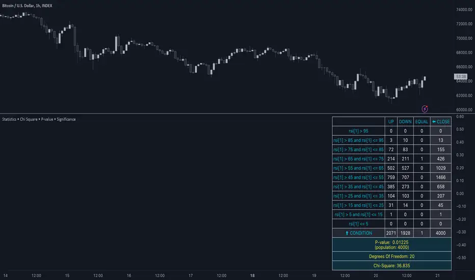
Statistics • Chi Square • P-value • SignificanceThe Statistics • Chi Square • P-value • Significance publication aims to provide a tool for combining different conditions and checking whether the outcome is significant using the Chi-Square Test and P-value.
🔶 USAGE
The basic principle is to compare two or more groups and check the results of a query test, such as asking men and women whether they want to see a romantic or non-romantic movie.
–––––––––––––––––––––––––––––––––––––––––––––
| | ROMANTIC | NON-ROMANTIC | ⬅︎ MOVIE |
–––––––––––––––––––––––––––––––––––––––––––––
| MEN | 2 | 8 | 10 |
–––––––––––––––––––––––––––––––––––––––––––––
| WOMEN | 7 | 3 | 10 |
–––––––––––––––––––––––––––––––––––––––––––––
|⬆︎ SEX | 10 | 10 | 20 |
–––––––––––––––––––––––––––––––––––––––––––––
We calculate the Chi-Square Formula, which is:
Χ² = Σ ( (Observed Value − Expected Value)² / Expected Value )
In this publication, this is:
chiSquare = 0.
for i = 0 to rows -1
for j = 0 to colums -1
observedValue = aBin.get(i).aFloat.get(j)
expectedValue = math.max(1e-12, aBin.get(i).aFloat.get(colums) * aBin.get(rows).aFloat.get(j) / sumT) //Division by 0 protection
chiSquare += math.pow(observedValue - expectedValue, 2) / expectedValue
Together with the 'Degree of Freedom', which is (rows − 1) × (columns − 1) , the P-value can be calculated.
In this case it is P-value: 0.02462
A P-value lower than 0.05 is considered to be significant. Statistically, women tend to choose a romantic movie more, while men prefer a non-romantic one.
Users have the option to choose a P-value, calculated from a standard table or through a math.ucla.edu - Javascript-based function (see references below).
Note that the population (10 men + 10 women = 20) is small, something to consider.
Either way, this principle is applied in the script, where conditions can be chosen like rsi, close, high, ...
🔹 CONDITION
Conditions are added to the left column ('CONDITION')
For example, previous rsi values (rsi ) between 0-100, divided in separate groups
🔹 CLOSE
Then, the movement of the last close is evaluated
UP when close is higher then previous close (close )
DOWN when close is lower then previous close
EQUAL when close is equal then previous close
It is also possible to use only 2 columns by adding EQUAL to UP or DOWN
UP
DOWN/EQUAL
or
UP/EQUAL
DOWN
In other words, when previous rsi value was between 80 and 90, this resulted in:
19 times a current close higher than previous close
14 times a current close lower than previous close
0 times a current close equal than previous close
However, the P-value tells us it is not statistical significant.
NOTE: Always keep in mind that past behaviour gives no certainty about future behaviour.
A vertical line is drawn at the beginning of the chosen population (max 4990)
Here, the results seem significant.
🔹 GROUPS
It is important to ensure that the groups are formed correctly. All possibilities should be present, and conditions should only be part of 1 group.
In the example above, the two top situations are acceptable; close against close can only be higher, lower or equal.
The two examples at the bottom, however, are very poorly constructed.
Several conditions can be placed in more than 1 group, and some conditions are not integrated into a group. Even if the results are significant, they are useless because of the group formation.
A population count is added as an aid to spot errors in group formation.
In this example, there is a discrepancy between the population and total count due to the absence of a condition.
The results when rsi was between 5-25 are not included, resulting in unreliable results.
🔹 PRACTICAL EXAMPLES
In this example, we have specific groups where the condition only applies to that group.
For example, the condition rsi > 55 and rsi <= 65 isn't true in another group.
Also, every possible rsi value (0 - 100) is present in 1 of the groups.
rsi > 15 and rsi <= 25 28 times UP, 19 times DOWN and 2 times EQUAL. P-value: 0.01171
When looking in detail and examining the area 15-25 RSI, we see this:
The population is now not representative (only checking for RSI between 15-25; all other RSI values are not included), so we can ignore the P-value in this case. It is merely to check in detail. In this case, the RSI values 23 and 24 seem promising.
NOTE: We should check what the close price did without any condition.
If, for example, the close price had risen 100 times out of 100, this would make things very relative.
In this case (at least two conditions need to be present), we set 1 condition at 'always true' and another at 'always false' so we'll get only the close values without any condition:
Changing the population or the conditions will change the P-value.
In the following example, the outcome is evaluated when:
close value from 1 bar back is higher than the close value from 2 bars back
close value from 1 bar back is lower/equal than the close value from 2 bars back
Or:
close value from 1 bar back is higher than the close value from 2 bars back
close value from 1 bar back is equal than the close value from 2 bars back
close value from 1 bar back is lower than the close value from 2 bars back
In both examples, all possibilities of close against close are included in the calculations. close can only by higher, equal or lower than close
Both examples have the results without a condition included (5 = 5 and 5 < 5) so one can compare the direction of current close.
🔶 NOTES
• Always keep in mind that:
Past behaviour gives no certainty about future behaviour.
Everything depends on time, cycles, events, fundamentals, technicals, ...
• This test only works for categorical data (data in categories), such as Gender {Men, Women} or color {Red, Yellow, Green, Blue} etc., but not numerical data such as height or weight. One might argue that such tests shouldn't use rsi, close, ... values.
• Consider what you're measuring
For example rsi of the current bar will always lead to a close higher than the previous close, since this is inherent to the rsi calculations.
• Be careful; often, there are na -values at the beginning of the series, which are not included in the calculations!
• Always keep in mind considering what the close price did without any condition
• The numbers must be large enough. Each entry must be five or more. In other words, it is vital to make the 'population' large enough.
• The code can be developed further, for example, by splitting UP, DOWN in close UP 1-2%, close UP 2-3%, close UP 3-4%, ...
• rsi can be supplemented with stochRSI, MFI, sma, ema, ...
🔶 SETTINGS
🔹 Population
• Choose the population size; in other words, how many bars you want to go back to. If fewer bars are available than set, this will be automatically adjusted.
🔹 Inputs
At least two conditions need to be chosen.
• Users can add up to 11 conditions, where each condition can contain two different conditions.
🔹 RSI
• Length
🔹 Levels
• Set the used levels as desired.
🔹 Levels
• P-value: P-value retrieved using a standard table method or a function.
• Used function, derived from Chi-Square Distribution Function; JavaScript
LogGamma(Z) =>
S = 1
+ 76.18009173 / Z
- 86.50532033 / (Z+1)
+ 24.01409822 / (Z+2)
- 1.231739516 / (Z+3)
+ 0.00120858003 / (Z+4)
- 0.00000536382 / (Z+5)
(Z-.5) * math.log(Z+4.5) - (Z+4.5) + math.log(S * 2.50662827465)
Gcf(float X, A) => // Good for X > A +1
A0=0., B0=1., A1=1., B1=X, AOLD=0., N=0
while (math.abs((A1-AOLD)/A1) > .00001)
AOLD := A1
N += 1
A0 := A1+(N-A)*A0
B0 := B1+(N-A)*B0
A1 := X*A0+N*A1
B1 := X*B0+N*B1
A0 := A0/B1
B0 := B0/B1
A1 := A1/B1
B1 := 1
Prob = math.exp(A * math.log(X) - X - LogGamma(A)) * A1
1 - Prob
Gser(X, A) => // Good for X < A +1
T9 = 1. / A
G = T9
I = 1
while (T9 > G* 0.00001)
T9 := T9 * X / (A + I)
G := G + T9
I += 1
G *= math.exp(A * math.log(X) - X - LogGamma(A))
Gammacdf(x, a) =>
GI = 0.
if (x<=0)
GI := 0
else if (x
Chisqcdf = Gammacdf(Z/2, DF/2)
Chisqcdf := math.round(Chisqcdf * 100000) / 100000
pValue = 1 - Chisqcdf
🔶 REFERENCES
mathsisfun.com, Chi-Square Test
Chi-Square Distribution Function
지표 및 전략
Trading Activity Index (Zeiierman)█ Overview
Trading Activity Index (Zeiierman) is a volume-based market activity meter that transforms dollar-volume into a smooth, normalized “activity index.”
It highlights when market participation is unusually low or high with a dynamic color gradient:
Light Blue → Low Activity (thin participation, low liquidity conditions)
Red/Orange → High Activity (active markets, large trades flowing in)
Additional percentile bands (20/40/60/80%) give context, helping you see whether the current activity level is in the bottom quintile, mid-range, or near historical extremes.
█ How It Works
⚪ Dollar Volume Transformation
Each bar, dollar volume is computed:
float dlrVol = close * volume
float dlrVolAvg = ta.sma(dlrVol, len_form)
Dollar volume = price × volume, smoothed by a configurable SMA window.
The result is log-transformed, compressing large outliers for a more stable signal.
⚪ Rolling Percentiles & Ranking
The log-dollar-volume series is compared to its rolling history (len_hist bars):
float p20 = ta.percentile_linear_interpolation(vscale, len_hist, 20)
float p40 = ta.percentile_linear_interpolation(vscale, len_hist, 40)
float p60 = ta.percentile_linear_interpolation(vscale, len_hist, 60)
float p80 = ta.percentile_linear_interpolation(vscale, len_hist, 80)
A normalized rank (0–1) is produced to color the main Trading Activity line.
█ How to Use
⚪ Detect High-Impact Sessions
Quickly see if today’s session is active or quiet relative to its own history — great for filtering setups that need activity.
⚪ Spot Breakouts & Traps
Combine with price action:
High activity near breakouts = strong follow-through likely.
Low activity breakouts = vulnerable to fake-outs.
⚪ Market Regime Context
Percentile bands help you assess whether participation is building up, in the middle of the range, or drying out — valuable for timing mean-reversion trades.
Above 80th percentile (red/orange) → Market is highly active, breakout trades and trend strategies are favored.
Below 20th percentile (light blue) → Market is quiet; fade moves or wait for expansion.
Watch transitions from blue → orange as a signal of growing institutional participation.
█ Settings
Formation Window (bars) – Number of bars used to average dollar volume before log transform.
History Window (bars) – Lookback period for percentile calculations and rank normalization.
-----------------
Disclaimer
The content provided in my scripts, indicators, ideas, algorithms, and systems is for educational and informational purposes only. It does not constitute financial advice, investment recommendations, or a solicitation to buy or sell any financial instruments. I will not accept liability for any loss or damage, including without limitation any loss of profit, which may arise directly or indirectly from the use of or reliance on such information.
All investments involve risk, and the past performance of a security, industry, sector, market, financial product, trading strategy, backtest, or individual's trading does not guarantee future results or returns. Investors are fully responsible for any investment decisions they make. Such decisions should be based solely on an evaluation of their financial circumstances, investment objectives, risk tolerance, and liquidity needs.

Expected Value Monte CarloI created this indicator after noticing that there was no Expected Value indicator here on TradingView.
The EVMC provides statistical Expected Value to what might happen in the future regarding the asset you are analyzing.
It uses 2 quantitative methods:
Historical Backtest to ground your analysis in long-term, factual data.
Monte Carlo Simulation to project a cone of probable future outcomes based on recent market behavior.
This gives you a data-driven edge to quantify risk, and make more informed trading decisions.
The indicator includes:
Dual analysis: Combines historical probability with forward-looking simulation.
Quantified projections: Provides the Expected Value ($ and %), Win Rate, and Sharpe Ratio for both methods.
Asset-aware: Automatically adjusts its calculations for Stocks (252 trading days) and Crypto (365 days) for mathematical accuracy.
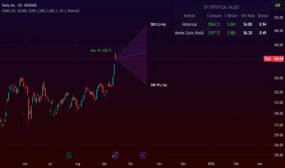
The projection cone shows the mean expected path and the +/- 1 standard deviation range of outcomes.
No repainting
Calculation:
1. Historical Expected Value:
This is a systematic backtest over thousands of bars. It calculates the return Rᵢ for N past trades (buy-and-hold). The Historical EV is the simple average of these returns, giving a baseline performance measure.
Historical EV % = (Σ Rᵢ) / N
2. Monte Carlo Projection:
This projection uses the Geometric Brownian Motion (GBM) model to simulate thousands of future price paths based on the market's recent behavior.
It first measures the drift (μ), or recent trend, and volatility (σ), or recent risk, from the Projection Lookback period. It then projects a final return for each simulation using the core GBM formula:
Projected Return = exp( (μ - σ²/2)T + σ√T * Z ) - 1
(Where T is the time horizon and Z is a random variable for the simulation.)
The purple line on the chart is the average of all simulated outcomes (the Monte Carlo EV). The cone represents one standard deviation of those outcomes.
The dashed lines represent one standard deviation (+/- 1σ) from the average, forming a cone of probable outcomes. Roughly 68% of the simulated paths ended within this cone.
This projection answers the question: "If the recent trend and volatility continue, where is the price most likely to go?"
Here's how to read the indicator
Expected Value ($/%): Is my average trade profitable?
Win Rate: How often can I expect to be right?
Sharpe Ratio: Am I being adequately compensated for the risk I'm taking?
User Guide
Max trade duration (bars): This is your analysis timeframe. Are you interested in the probable outcome over the next month (21 bars), quarter (63 bars), or year (252 bars)?
Position size ($): Set this to your typical trade size to see the Expected Value in real dollar terms.
Projection lookback (bars): This is the most important input for the Monte Carlo model. A short lookback (e.g., 50) makes the projection highly sensitive to recent momentum. Use this to identify potential recency bias. A long lookback (e.g., 252) provides a more stable, long-term projection of trend and volatility.
Historical Lookback (bars): For the historical backtest, more data is always better. Use the maximum that your TradingView plan allows for the most statistically significant results.
Use TP/SL for Historical EV: Check this box to see how the historical performance would have changed if you had used a simple Take Profit and Stop Loss, rather than just holding for the full duration.
I hope you find this indicator useful and please let me know if you have any suggestions. 😊
Liquidity Void Detector (Zeiierman)█ Overview
Liquidity Void Detector (Zeiierman) is an oscillator highlighting inefficient price displacements under low participation. It measures the most recent price move (standardized return) and amplifies it only when volume is below its own trend.
Positive readings ⇒ strong up-move on low volume → potential Buy-Side Imbalance (void below) that often refills.
Negative readings ⇒ strong down-move on low volume → potential Sell-Side Imbalance (void above) that often refills.
This tool provides a quantitative “void” proxy: when price travels far with unusually thin volume, the move is flagged as likely inefficient and prone to mean-reversion/mitigation.
█ How It Works
⚪ Volume Shock (Participation Filter)
Each bar, volume is compared to a rolling baseline. This is then z-scored.
// Volume Shock calculation
volTrend = ta.sma(volume, L)
vs = (volume > 0 and volTrend > 0) ? math.log(volume) - math.log(volTrend) : na
vsZ = zScore(vs, vzLen) // z-scored volume shock
lowVS = (vsZ <= vzThr) // low-volume condition
Bars with VolShock Z ≤ threshold are treated as low-volume (thin).
⚪ Prior Return Extremeness
The 1-bar log return is computed and z-scored.
// Prior return extremeness
r1 = math.log(close / close )
retZ = zScore(r1, rLen) // z-scored prior return
This shows whether the latest move is unusually large relative to recent history.
⚪ Void Oscillator
The oscillator is:
// Oscillator construction
weight = lowVS ? 1.0 : fadeNoLow
osc = retZ * weight
where Weight = 1 when volume is low, otherwise fades toward a user-set factor (0–1).
Osc > 0: up-move emphasized under low volume ⇒ Buy-Side Imbalance.
Osc < 0: down-move emphasized under low volume ⇒ Sell-Side Imbalance.
█ Why Use It
⚪ Targets Inefficient Moves
By filtering for low participation, the oscillator focuses on moves most likely driven by thin books/noise trading, which are statistically more likely to retrace.
⚪ Simple, Robust Logic
No need for tick data or order-book depth. It derives a practical void proxy from OHLCV, making it portable across assets and timeframes.
⚪ Complements Price-Action Tools
Use alongside FVG/imbalance zones, key levels, and volume profile to prioritize voids that carry the highest reversal probability.
█ How to Use
Sell-Side Imbalance = aggressive sell move (price goes down on low volume) → expect price to move up to fill it.
Buy-Side Imbalance = aggressive buy move (price goes up on low volume) → expect price to move down to fill it.
█ Settings
Volume Baseline Length — Bars for the volume trend used in VolShock. Larger = smoother baseline, fewer low-volume flags.
Vol Shock Z-Score Lookback — Bars to standardize VolShock; larger = smoother, fewer extremes.
Low-Volume Threshold (VolShock Z ≤) — Defines “thin participation.” Typical: −0.5 to −1.0.
Return Z-Score Lookback — Bars to standardize the 1-bar log return; larger = smoother “extremeness” measure.
Fade When Volume Not Low (0–1) — Weight applied when volume is not low. 0.00 = ignore non-low-volume bars entirely. 1.00 = treat volume condition as irrelevant (pure return extremeness).
Upper Threshold (Osc ≥) — Trigger for Sell-Side Imbalance (void below).
Lower Threshold (Osc ≤) — Trigger for Buy-Side Imbalance (void above).
-----------------
Disclaimer
The content provided in my scripts, indicators, ideas, algorithms, and systems is for educational and informational purposes only. It does not constitute financial advice, investment recommendations, or a solicitation to buy or sell any financial instruments. I will not accept liability for any loss or damage, including without limitation any loss of profit, which may arise directly or indirectly from the use of or reliance on such information.
All investments involve risk, and the past performance of a security, industry, sector, market, financial product, trading strategy, backtest, or individual's trading does not guarantee future results or returns. Investors are fully responsible for any investment decisions they make. Such decisions should be based solely on an evaluation of their financial circumstances, investment objectives, risk tolerance, and liquidity needs.

DeltaFlow Volume Profile [BigBeluga]🔵 OVERVIEW
The DeltaFlow Volume Profile builds a compact volume profile next to price and enriches every bin with flow context : bullish vs. bearish participation (%), a per-bin Delta % , an optional Delta Heat Map , and a PoC band with the bin’s absolute volume. This lets you see not just where volume clustered, but who (buyers or sellers) dominated inside each price slice.
🔵 CONCEPTS
Binned Volume Profile : Price range over a user-defined LookBack is split into Bins ; each bin aggregates traded volume.
Bull/Bear Split : Within every bin, volume is separated by candle direction into Bull Volume and Bear Volume , then normalized to % of the bin’s displayed size.
Delta % : The difference between Bull % and Bear % for the bin. Positive = buyer dominance; negative = seller dominance.
Delta Heat Map : Bin background shading that scales with both total volume strength and delta bias.
PoC (Point of Control) : The most significant bin gets a PoC band and a label with its absolute volume.
🔵 FEATURES
Profile with Flow : A clean horizontal volume bar per bin plus stacked Bull % and Bear % .
Per-Bin Delta Label : A readable “Δ xx%” tag at the start of each bin shows dominance at a glance.
Delta Heat Map : Optional gradient that intensifies with higher volume and stronger delta.
PoC Highlight : Optional PoC band colored separately, labeled with absolute volume (e.g., “1.23M”).
Configurable Inputs : LookBack, number of Bins (10–100), toggles for Delta, Heat Map, Volume Bars, and PoC color.
Readable Colors : Separate inputs for bullish (volume +) and bearish (volume –) hues.
🔵 HOW TO USE
Set the window : Choose LookBack and Bins to balance detail vs. performance (more bins = finer resolution).
Enable “Volume Bars” to display the bull/bear split as two stacked percent bars inside each bin.
High Bull % near support → constructive demand.
High Bear % near resistance → active supply.
Use Δ labels (toggle “Delta”) to quickly spot bins with clear buyer/seller control; combine with price position for confluence.
Turn on Delta Heat Map to prioritize areas with both large volume and strong imbalance.
Watch the PoC : The PoC band marks the most traded (and often magnet) level; its label shows absolute size for context.
Trade ideas :
Breakout continuation when Δ stays positive across consecutive upper bins.
Reversion risk when price enters a large bearish-Δ cluster below.
Manage risk around the PoC; reactions there can be sharp.
🔵 CONCLUSION
DeltaFlow Volume Profile upgrades a classic profile with flow intelligence. The bull/bear split, explicit Δ %, heat-weighted backdrop, and PoC volume label make dominant participation and key price shelves obvious. Use it to filter levels, time entries with imbalance, and validate breakouts or fades with objective volume-flow evidence.

Volume by Time [LuxAlgo]The Volume by Time indicator collects volume data for every point in time over the day and displays the average volume of the specific dataset collected at each respective bar.
The indicator overlays the current volume and the historical average to allow for better comparisons.
🔶 USAGE
Throughout the day, the volume of every bar is stored in groups organized by the time when each bar occurred.
Over time, the datasets accumulate, and from that, we can simply determine the average value at each specific time of the day.
The display is a histogram style, which consists of hollow bars and solid filled columns.
-Hollow bars represent the average volume at that time of the day.
-Solid columns display the current volume from the current bar.
By default, the entire history of data is used, but if desired, the number of days under analysis can be specified to provide a more relevant point of view.
A readout of the number of days being analyzed can be seen in the status bar at any time.
Note: Due to partial sessions, it is typical to see this value change throughout the day; this is simply due to the fact that not every trading session has the exact same schedule 100% of the time.
The analysis type can also be specified; these can be either Average (Default) or Median.
Additionally, a Bi-directional can be toggled for a distinct difference between upwards volume and downwards volume.
🔶 SETTINGS
Analysis Type: Choose between Average or Median analysis modes.
Length (Days): Set the number of days to use for analysis. Set to 0 for full data (Default 0).
Bi-Directional Toggle: Toggle between one-sided or two-sided display.

FlowScope [Hapharmonic]FlowScope: Uncover the Market's True Intent 🔬
Ever wished you could look inside the candles and see where the real action is happening? FlowScope is your microscope for the market's flow, designed to give you a powerful edge by revealing the volume distribution that price action alone can't show you.
Instead of just looking at the open, high, low, and close, FlowScope lets you dive deeper into the market's auction process. It groups candles together and builds a detailed Volume Profile for that period, showing you exactly where the trading happened and revealing the story behind the price action.
Let's explore how you can use it to gain a powerful new edge.
🧐 Core Concept: How It Works
At its heart, FlowScope does three key things:
It Groups Candles: You decide how many candles to group together. For example, setting " Group Candles " to 4 on a 5-minute chart effectively gives you a detailed 20-minute candle and profile. This helps you see the bigger picture and filter out market noise.
It Builds a Volume Profile: For each group, FlowScope analyzes the volume at every single price level. It then displays this as a horizontal histogram (we call this a "footprint" or profile). Longer bars mean more volume was traded at that price, indicating a "fair" price or an area of acceptance. Shorter bars mean price moved through quickly, indicating rejection.
It Creates a Custom "Grouped Candle": To summarize the group's overall price action, FlowScope draws a single, custom candle representing the entire group's:
Open: The open of the first candle in the group.
High: The absolute highest price reached within the group.
Low: The absolute lowest price reached within the group.
Close: The close of the last candle in the group.
This gives you a crystal-clear view of the group's net result, free from the back-and-forth noise of the individual candles inside it.
Below are some of the stunning preset color palettes you can choose from to customize your view:
🚀 How to Use: Practical Applications
FlowScope isn't just for looking pretty; it's a powerful analysis tool. Here are a few ways to integrate it into your trading:
Identify High-Volume Nodes (HVNs): Look for the longest bars in the profile. These are price levels where the market spent the most time and traded the most volume. HVNs often act as powerful "magnets" for price, becoming key areas of support and resistance.
Spot Low-Volume Nodes (LVNs): These are areas with very short bars or gaps in the profile. They represent price levels that the market moved through quickly and inefficiently. If price returns to an LVN, it's likely to move through it quickly again.
Analyze the Summary Box: This is where the real magic happens! ✨
Total Volume (Σ): The total volume for the entire group.
Buy (B) vs. Sell (S) Volume: FlowScope analyzes the lower timeframe action to estimate the buying and selling pressure that made up the total volume. Is a big red candle mostly aggressive selling, or was it just a lack of buyers? The B/S data gives you clues. A high-volume candle with nearly 50/50 buy/sell pressure might indicate absorption or a potential reversal.
Use the Grouped Candle for Clarity: Is the market in a clear uptrend, or is it just choppy? The grouped candle can give you a much clearer signal. A series of strong, green grouped candles shows much more conviction than a mix of small green and red candles.
⚙️ Settings & Customization
This is where you can truly make FlowScope your own. Let's walk through each setting.
Profile Settings
Group Candles: The number of standard chart candles you want to combine into a single FlowScope profile. A setting of 1 will analyze every single bar. A higher number gives you a broader market view. When Group Candles is set to 5, the data from the 5 individual candles are combined, and the volume is calculated accordingly.
Max Profile Boxes: This setting is more than just a number; it's a smart limit that ensures your profiles are always readable and relevant to the current market conditions.
Adaptive Sizing (The Ideal Goal): FlowScope first tries to create the perfect profile by making each volume box's height proportional to the current market volatility. It calculates an "ideal" box height based on the Average True Range ( ATR / 10 ). This is powerful because it automatically adapts: you get smaller, more detailed boxes in quiet, low-volatility markets, and larger, clearer boxes in volatile, fast-moving markets.
The Safety Cap (Your Setting): However, what if you group several candles during a massive price move? The price range could be huge! If we only used the small, ATR-based box height, you might end up with hundreds of tiny, unreadable boxes. This is where your Max Profile Boxes setting (defaulting to 50) comes in. It acts as a maximum detail cap . If the adaptive, volatility-based calculation determines that it would need more boxes than your setting (e.g., more than 50), the indicator will override it. It will then simply divide the entire price range of the group into exactly the number of boxes you specified (e.g., 50).
In short: You are setting the maximum allowable detail. FlowScope intelligently adapts the profile's granularity below that limit based on market volatility, ensuring you always get a clear and meaningful picture.
Style
Show Profile BG: A simple toggle to show or hide the faint background color behind the volume bars. Turning it off can create a cleaner look.
Color Mode: This dropdown controls how the volume profile text is colored.
Custom Gradient: This mode uses the three custom colors you select in the "Profile Colors" section to create a beautiful gradient across the profile.
Candle Color: This mode colors the profile based on whether the grouped candle was bullish (green) or bearish (red). The color will be a gradient, with the most intense color applied to the box with the highest volume; the colors of the other boxes will fade out from that point. It's a great way to see the profile's "mood" at a glance.
Profile Colors 🎨
Use Preset Palette: This is the master switch!
If checked: You can choose from 10 stunning, pre-designed color palettes from the Palette dropdown. The custom color pickers below will be disabled.
If unchecked (Default): The Palette dropdown will be disabled, and you can now choose your own three colors for the gradient.
Palette: (Only active when "Use Preset Palette" is checked) . Choose from 10 luxurious, eye-catching color schemes like "Solar Flare" or "Deep Space" to instantly change the look and feel of your chart.
Low Price / Mid Price / High Price: (Only active when "Use Preset Palette" is unchecked) . These three color pickers allow you to design your own unique gradient for the Custom Gradient color mode.
Candle Display
These settings control the custom "Grouped Candle" that summarizes the profile. When using the "Show Custom Candle" feature, you should change the chart's candlestick display to Bars for a cleaner view.
Show Custom Candle: This is the main toggle. When you check this box, the original chart candles will be hidden, and your custom FlowScope candle will be displayed instead. This custom candle is intentionally small to ensure it does not visually overlap with the volume profile boxes.
Show Body: (Only active when "Show Custom Candle" is checked) . Toggles the visibility of the candle's body.
Wick Width & Body Width: (Only active when "Show Custom Candle" is checked) . These sliders let you control the thickness of the wick and body lines to match your personal style.
Up Color / Down Color: (Only active when "Show Custom Candle" is checked) . Choose the colors for your bullish and bearish custom candles.
Experiment with the settings, find a style that works for you, and start seeing the market in a whole new light.
Happy trading! 📈😊

VWAP Price ChannelVWAP Price Channel cuts the crust off of a traditional price channel (Donchian Channel) by anchoring VWAPs at the highs and lows. By doing this, the flat levels, characteristic of traditional Donchian Channels, are no more!
Author's Note: This indicator is formed with no inherent use, and serves solely as a thought experiment.
> Concept
I would be hesitant to call this a "predictive" indicator, however the behavior of it would suggest it could be considered at least partially predictive
Essentially, the Anchored VWAPs creates something from otherwise nothing.
While the DC upper or lower values are staying flat, the VWAPs improvise based on price and volume to project a level that may be a better representation of where future highs or lows may settle.
Visually, this looks like we have cut off the corners of the Donchian Channel.
Note: Notice how we are calculating values before the corners are realized.
> Implementation
While this is only a concept indicator, The specific application I've gone with for this, is a sort of supertrend-ish display (A Trend Flipping Trailing Stop Loss).
The script uses basic logic to create a trend direction, and then displays the Anchored VWAPs as a form of trailing stop loss.
While "In Trend", the script fills in the area between the VWAP and Price in the direction of trend.
When new highs or lows are made while in trend, the opposite VWAP will start to generate at the new highs or lows. These happen on every new high or low, so they are not indicating the trend shift, but could be interpreted as breakout levels for the current trend direction in order for continuation.
Note: All values are drawn live, but when using higher timeframes, there is a natural calculation discrepancy when using live data vs. historical.
> Technicals
In this script, I'm simply detecting new highs or lows from the DC and using those as the anchor frequency on the built-in VWAP function.
So each time a new high or low is made based on DC, the VWAP function re-anchors to the high or low of the candle.
Past that, I have implemented some logic in order to account for a common occurrence I faced during development.
Frequently, the price would outpace the anchored VWAP, so we would end up with the VWAP being further from price than the actual DC upper or lower.
Due to this, what I have ended up with was a third value which, rather than switching between raw VWAP values and DC values, it adjusts the value based on the change in the VWAP value.
This can be simply thought of as a "Start + Change" type of setup.
By doing this, I can use the change values from the actual anchored VWAP, and under normal conditions, this will also be the true VWAP value.
However, situationally, I am able to update the start value which we're applying the VWAP change to.
In other words, when these situations happen, the VWAP change is added to the new (closer to price) DC value.
The specific trend logic being used is nothing fancy at all, we are simply checking if a new high or low is created and setting the trend in that direction.
This is in line with some traditional DC Strategies.
To those who made it here,
Just remember:
The chart may be ugly, but it's the fastest analysis of the data you can get.
Nicer displays often come at the hidden cost of latency.
You have to shoot your shot to make it.
Choose 2: Fast, Clean, Useful
Enjoy!

Fibonacci Sequence Circles [BigBeluga]🔵 Overview
The Fibonacci Sequence Circles is a unique and visually intuitive indicator designed for the TradingView platform. It combines the principles of the Fibonacci sequence with geometric circles to help traders identify potential support and resistance levels, as well as price expansion zones. The indicator dynamically anchors to key price points, such as pivot highs, pivot lows, or timeframe changes (daily, weekly, monthly), and generates Fibonacci-based circles around these anchor points.
⚠️For proper indicators visualization use simple not logarithmic chart
🔵 Key Features
Customizable Anchor Points : The indicator can be anchored to Pivot Highs , Pivot Lows , or timeframe changes ( Daily, Weekly, Monthly ), making it adaptable to various trading strategies.
Fibonacci Sequence Logic : The circles are generated using the Fibonacci sequence, where the diameter of each circle is the sum of the diameters of the two preceding circles.
first = start_val
secon = start_val + int(start_val/2)
three = first + secon
four = secon + three
five = three + four
six = four + five
seven = five + six
eight = six + seven
nine = seven + eight
ten = eight + nine
Adjustable Start Value : Traders can modify the starting value of the sequence to scale the circles larger or smaller, ensuring they fit the current price action.
Color Customization : Each circle can be individually enabled or disabled, and its color can be customized for better visual clarity.
Visual Labels : The diameter of each circle (in bars) is displayed next to the circle, providing additional context for analysis.
🔵 Usage
Step 1: Set the Anchor Point - Choose the anchor type ( Pivot High, Pivot Low, Daily, Weekly, Monthly ) to define the center of the Fibonacci circles.
Step 2: Adjust the Start Value - Modify the starting value of the Fibonacci sequence to scale the circles according to the price action.
Step 3: Customize Circle Colors - Enable or disable specific circles and adjust their colors for better visualization.
Step 4: Analyze Price Action - Use the circles to identify potential support/resistance levels, price expansion zones, or trend continuation areas.
Step 5: Combine with Other Tools - Enhance your analysis by combining the indicator with other technical tools like trendlines, moving averages, or volume indicators.
The Fibonacci Sequence Circles is a powerful and flexible tool for traders who rely on Fibonacci principles and geometric patterns. Its ability to anchor to key price points and dynamically scale based on market conditions makes it suitable for various trading styles and timeframes. Whether you're a day trader or a long-term investor, this indicator can help you visualize and anticipate price movements with greater precision.

ATAI Volume Pressure Analyzer V 1.0 — Pure Up/DownATAI Volume Pressure Analyzer V 1.0 — Pure Up/Down
Overview
Volume is a foundational tool for understanding the supply–demand balance. Classic charts show only total volume and don’t tell us what portion came from buying (Up) versus selling (Down). The ATAI Volume Pressure Analyzer fills that gap. Built on Pine Script v6, it scans a lower timeframe to estimate Up/Down volume for each host‑timeframe candle, and presents “volume pressure” in a compact HUD table that’s comparable across symbols and timeframes.
1) Architecture & Global Settings
Global Period (P, bars)
A single global input P defines the computation window. All measures—host‑TF volume moving averages and the half‑window segment sums—use this length. Default: 55.
Timeframe Handling
The core of the indicator is estimating Up/Down volume using lower‑timeframe data. You can set a custom lower timeframe, or rely on auto‑selection:
◉ Second charts → 1S
◉ Intraday → 1 minute
◉ Daily → 5 minutes
◉ Otherwise → 60 minutes
Lower TFs give more precise estimates but shorter history; higher TFs approximate buy/sell splits but provide longer history. As a rule of thumb, scan thin symbols at 5–15m, and liquid symbols at 1m.
2) Up/Down Volume & Derived Series
The script uses TradingView’s library function tvta.requestUpAndDownVolume(lowerTf) to obtain three values:
◉ Up volume (buyers)
◉ Down volume (sellers)
◉ Delta (Up − Down)
From these we define:
◉ TF_buy = |Up volume|
◉ TF_sell = |Down volume|
◉ TF_tot = TF_buy + TF_sell
◉ TF_delta = TF_buy − TF_sell
A positive TF_delta indicates buyer dominance; a negative value indicates selling pressure. To smooth noise, simple moving averages of TF_buy and TF_sell are computed over P and used as baselines.
3) Key Performance Indicators (KPIs)
Half‑window segmentation
To track momentum shifts, the P‑bar window is split in half:
◉ C→B: the older half
◉ B→A: the newer half (toward the current bar)
For each half, the script sums buy, sell, and delta. Comparing the two halves reveals strengthening/weakening pressure. Example: if AtoB_delta < CtoB_delta, recent buying pressure has faded.
[ 4) HUD (Table) Display /i]
Colors & Appearance
Two main color inputs define the theme: a primary color and a negative color (used when Δ is negative). The panel background uses a translucent version of the primary color; borders use the solid primary color. Text defaults to the primary color and flips to the negative color when a block’s Δ is negative.
Layout
The HUD is a 4×5 table updated on the last bar of each candle:
◉ Row 1 (Meta): indicator name, P length, lower TF, host TF
◉ Row 2 (Host TF): current ↑Buy, ↓Sell, ΔDelta; plus Σ total and SMA(↑/↓)
◉ Row 3 (Segments): C→B and B→A blocks with ↑/↓/Δ
◉ Rows 4–5: reserved for advanced modules (Wings, α/β, OB/OS, Top
5) Advanced Modules
5.1 Wings
“Wings” visualize volume‑driven movement over C→B (left wing) and B→A (right wing) with top/bottom lines and a filled band. Slopes are ATR‑per‑bar normalized for cross‑symbol/TF comparability and converted to angles (degrees). Coloring mirrors HUD sign logic with a near‑zero threshold (default ~3°):
◉ Both lines rising → blue (bullish)
◉ Both falling → red (bearish)
◉ Mixed/near‑zero → gray
Left wing reflects the origin of the recent move; right wing reflects the current state.
5.2 α / β at Point B
We compute the oriented angle between the two wings at the midpoint B:
β is the bottom‑arc angle; α = 360° − β is the top‑arc angle.
◉ Large α (>180°) or small β (<180°) flags meaningful imbalance.
◉ Intuition: large α suggests potential selling pressure; small β implies fragile support. HUD cells highlight these conditions.
5.3 OB/OS Spike
OverBought/OverSold (OB/OS) labels appear when directional volume spikes align with a 7‑oscillator vote (RSI, Stoch, %R, CCI, MFI, DeMarker, StochRSI).
◉ OB label (red): unusually high sell volume + enough OB votes
◉ OS label (teal): unusually high buy volume + enough OS votes
Minimum votes and sync window are user‑configurable; dotted connectors can link labels to the candle wick.
5.4 Top3 Volume Peaks
Within the P window the script ranks the top three BUY peaks (B1–B3) and top three SELL peaks (S1–S3).
◉ B1 and S1 are drawn as horizontal resistance (at B1 High) and support (at S1 Low) zones with adjustable thickness (ticks/percent/ATR).
◉ The HUD dedicates six cells to show ↑/↓/Δ for each rank, and prints the exact High (B1) and Low (S1) inline in their cells.
6) Reading the HUD — A Quick Checklist
◉ Meta: Confirm P and both timeframes (host & lower).
◉ Host TF block: Compare current ↑/↓/Δ against their SMAs.
◉ Segments: Contrast C→B vs B→A deltas to gauge momentum change.
◉ Wings: Right‑wing color/angle = now; left wing = recent origin.
◉ α / β: Look for α > 180° or β < 180° as imbalance cues.
◉ OB/OS: Note labels, color (red/teal), and the vote count.
◉Top3: Keep B1 (resistance) and S1 (support) on your radar.
Use these together to sketch scenarios and invalidation levels; never rely on a single signal in isolation.
[ 7) Example Highlights (What the table conveys) /i]
◉ Row 1 shows the indicator name, the analysis length P (default 55), and both TFs used for computation and display.
◉ B1 / S1 blocks summarize each side’s peak within the window, with Δ indicating buyer/seller dominance at that peak and inline price (B1 High / S1 Low) for actionable levels.
◉ Angle cells for each wing report the top/bottom line angles vs. the horizontal, reflecting the directional posture.
◉ Ranks B2/B3 and S2/S3 extend context beyond the top peak on each side.
◉ α / β cells quantify the orientation gap at B; changes reflect shifting buyer/seller influence on trend strength.
Together these visuals often reveal whether the “wings” resemble a strong, upward‑tilted arm supported by buyer volume—but always corroborate with your broader toolkit
8) Practical Tips & Tuning
◉ Choose P by market structure. For daily charts, 34–89 bars often works well.
◉ Lower TF choice: Thin symbols → 5–15m; liquid symbols → 1m.
◉ Near‑zero angle: In noisy markets, consider 5–7° instead of 3°.
◉ OB/OS votes: Daily charts often work with 3–4 votes; lower TFs may prefer 4–5.
◉ Zone thickness: Tie B1/S1 zone thickness to ATR so it scales with volatility.
◉ Colors: Feel free to theme the primary/negative colors; keep Δ<0 mapped to the negative color for readability.
Combine with price action: Use this indicator alongside structure, trendlines, and other tools for stronger decisions.
Technical Notes
Pine Script v6.
◉ Up/Down split via TradingView/ta library call requestUpAndDownVolume(lowerTf).
◉ HUD‑first design; drawings for Wings/αβ/OBOS/Top3 align with the same sign/threshold logic used in the table.
Disclaimer: This indicator is provided solely for educational and analytical purposes. It does not constitute financial advice, nor is it a recommendation to buy or sell any security. Always conduct your own research and use multiple tools before making trading decisions.

Market Cap Landscape 3DHello, traders and creators! 👋
Market Cap Landscape 3D. This project is more than just a typical technical analysis tool; it's an exploration into what's possible when code meets artistry on the financial charts. It's a demonstration of how we can transcend flat, two-dimensional lines and step into a vibrant, three-dimensional world of data.
This project continues a journey that began with a previous 3D experiment, the T-Virus Sentiment, which you can explore here:
The Market Cap Landscape 3D builds on that foundation, visualizing market data—particularly crypto market caps—as a dynamic 3D mountain range. The entire landscape is procedurally generated and rendered in real-time using the powerful drawing capabilities of polyline.new() and line.new() , pushed to their creative limits.
This work is intended as a guide and a design example for all developers, born from the spirit of learning and a deep love for understanding the Pine Script™ language.
---
🧐 Core Concept: How It Works
The indicator synthesizes multiple layers of information into a single, cohesive 3D scene:
The Surface: The mountain range itself is a procedurally generated 3D mesh. Its peaks and valleys create a rich, textured landscape that serves as the canvas for our data.
Crypto Data Integration: The core feature is its ability to fetch market cap data for a list of cryptocurrencies you provide. It then sorts them in descending order and strategically places them onto the 3D surface.
The Summit: The highest point on the mountain is reserved for the asset with the #1 market cap in your list, visually represented by a flag and a custom emblem.
The Mountain Labels: The other assets are distributed across the mountainside, with their rank determining their general elevation. This creates an intuitive visual hierarchy.
The Leaderboard Pole: For clarity, a dedicated pole in the back-right corner provides a clean, ranked list of the symbols and their market caps, ensuring the data is always easy to read.
---
🧐 Example of adjusting the view
To evoke the feeling of flying over mountains
To evoke the feeling of looking at a mountain peak on a low plain
🧐 Example of predefined colors
---
🚀 How to Use
Getting started with the Market Cap Landscape 3D:
Add to Chart: Apply the "Market Cap Landscape 3D" indicator to your active chart.
Open Settings: Double-click anywhere on the 3D landscape or click the "Settings" icon next to the indicator's name.
Customize Your Crypto List: The most important setting is in the Crypto Data tab. In the "Symbols" text area, enter a comma-separated list of the crypto tickers you want to visualize (e.g., BTC,ETH,SOL,XRP ). The indicator supports up to 40 unique symbols.
> Important Note: This indicator exclusively uses TradingView's `CRYPTOCAP` data source. To find valid symbols, use the main symbol search bar on your chart. Type `CRYPTOCAP:` (including the colon) and you will see a list of available options. For example, typing `CRYPTOCAP:BTC` will confirm that `BTC` is a valid ticker for the indicator's settings. Using symbols that do not exist in the `CRYPTOCAP` index will result in a script error. or, to display other symbols, simply type CRYPTOCAP: (including the colon) and you will see a list of available options.
Adjust Your View: Use the settings in the Camera & Projection tab to rotate ( Yaw ), tilt ( Pitch ), and scale the landscape until you find a view you love.
Explore & Customize: Play with the color palettes, flag design, and other settings to make the landscape truly your own!
---
⚙️ Settings & Customization
This indicator is highly customizable. Here’s a breakdown of what each setting does:
#### 🪙 Crypto Data
Symbols: Enter the crypto tickers you want to track, separated by commas. The script automatically handles duplicates and case-insensitivity.
Show Market Cap on Mountain: When checked, it displays the full market cap value next to the symbol on the mountain. When unchecked, it shows a cleaner look with just the symbol and a colored circle background.
#### 📷 Camera & Projection
Yaw (°): Rotates the camera view horizontally (side to side).
Pitch (°): Tilts the camera view vertically (up and down).
Scale X, Y, Z: Stretches or compresses the landscape in width, depth, and height, respectively. Fine-tune these to get the perfect perspective.
#### 🏞️ Grid / Surface
Grid X/Y resolution: Controls the detail level of the 3D mesh. Higher values create a smoother surface but may use more resources.
Fill surface strips: Toggles the beautiful color gradient on the surface.
Show wireframe lines: Toggles the visibility of the grid lines.
Show nodes (markers): Toggles the small dots at each grid intersection point.
#### 🏔️ Peaks / Mountains
Fill peaks volume: Draws vertical lines on high peaks, giving them a sense of volume.
Fill peaks surface: Draws a cross-hatch pattern on the surface of high peaks.
Peak height threshold: Defines the minimum height for a peak to receive the fill effect.
Peak fill color/density: Customizes the appearance of the fill lines.
#### 🚩 Flags (3D)
Show Flag on Summit: A master switch to show or hide the flag and emblem entirely.
Flag height, width, etc.: Provides full control over the dimensions and orientation of the flag on the highest peak.
#### 🎨 Color Palette
Base Gradient Palette: Choose from 13 stunning, pre-designed color themes for the landscape, from the classic SUNSET_WAVE to vibrant themes like NEON_DREAM and OCEANIC .
#### 🛡️ Emblem / Badge Controls
This section gives you granular control over every element of the custom emblem on the flag. Tweak rotation, offsets, and scale to design your unique logo.
---
👨💻 Developer's Corner: Modifying the Core Logic
If you're a developer and wish to customize the indicator's core data source, this section is for you. The script is designed to be modular, making it easy to change what data is being ranked and visualized.
The heart of the data retrieval and ranking logic is within the f_getSortedCryptoData() function. Here’s how you can modify it:
1. Changing the Data Source (from Market Cap to something else):
The current logic uses request.security("CRYPTOCAP:" + syms.get(i), ...) to fetch market capitalization data. To change this, you need to modify this line.
Example: Ranking by RSI (14) on the Daily timeframe.
First, you'll need a function to calculate RSI. Add this function to the script:
f_getRSI(symbol, timeframe, length) =>
request.security(symbol, timeframe, ta.rsi(close, length))
Then, inside f_getSortedCryptoData() , find the `for` loop that populates the `caps` array and replace the `request.security` call:
// OLD LINE:
// caps.set(i, request.security("CRYPTOCAP:" + syms.get(i), timeframe.period, close))
// NEW LINE for RSI:
// Note: You'll need to decide how to format the symbol name (e.g., "BINANCE:" + syms.get(i) + "USDT")
caps.set(i, f_getRSI("BINANCE:" + syms.get(i) + "USDT", "D", 14))
2. Changing the Data Formatting:
The ranking values are formatted for display using the f_fmtCap() function, which currently formats large numbers into "M" (millions), "B" (billions), etc.
If you change the data source to something like RSI, you'll want to change the formatting. You can modify f_fmtCap() or create a new formatting function.
Example: Formatting for RSI.
// Modify f_fmtCap or create f_fmtRSI
f_fmtRSI(float v) =>
str.tostring(v, "#.##") // Simply format to two decimal places
Remember to update the calls to this function in the main drawing loop where the labels are created (e.g., str.format("{0}: {1}", crypto.symbol, f_fmtCap(crypto.cap)) ).
By modifying these key functions ( f_getSortedCryptoData and f_fmtCap ), you can adapt the Market Cap Landscape 3D to visualize and rank almost any dataset you can imagine, from technical indicators to fundamental data.
---
We hope you enjoy using the Market Cap Landscape 3D as much as we enjoyed creating it. Happy charting! ✨

Angled Volume Profile [Trendoscope]Volume profile is useful tool to understand the demand and supply zones on horizontal level. But, what if you want to measure the volume levels over trend line? In trending markets, the feature to measure volume over angled levels can be very useful for traders who use these measures. Here is an attempt to provide such tool.
🎲 How to use
🎯 Interactive input for selecting starting point and angle.
Upon loading the script, you will be prompted to select
Start time and price - this is a point which you can select by moving the maroon highlighted label.
End price - though this is shown as maroon bullet, this is price only input. Hence, when you click on the bullet, a horizontal line will appear. Users can move the line to use different End price.
Start and End price are used for identifying the angle at which volume profile need to be calculated. Whereas start time is used as starting time of the volume profile. Last bar of the chart is considered as ending bar.
🎯 Other settings.
From settings, users can select the colour of volume profile and style. Step multiplier defines the distance at which the profile lines needs to be drawn. Higher multiplier leads to less dense profile lines whereas lower multiplier leads to higher density of profile lines.
🎲 Limitations
🎯 Max 500 lines
Pinescript only allows max 500 lines on an indicator. Due to this, if we set very low multiplier - this can lead to more than 500 profile lines. Due to this some lines can get removed.
On the contrary, if multiplier is too high, then you will see very few lines which may not be meaningful.
Hence, it is important to select optimal multiplier based on your timeframe
🎯 No updates on new bar
Since the profile can spawn many bars, it is not possible to recalculate the whole volume profile when price creates new bars. Hence, there will not be visual update when new bars are created. But, to update the chart, users only need to make another movement of Start or ending point on interactive input.

Treasury Yields Heatmap [By MUQWISHI]▋ INTRODUCTION :
The “Treasury Yields Heatmap” generates a dynamic heat map table, showing treasury yield bond values corresponding with dates. In the last column, it presents the status of the yield curve, discerning whether it’s in a normal, flat, or inverted configuration, which determined by using Pearson's linear regression coefficient. This tool is built to offer traders essential insights for effectively tracking bond values and monitoring yield curve status, featuring the flexibility to input a starting period, timeframe, and select from a range of major countries' bond data.
_______________________
▋ OVERVIEW:
______________________
▋ YIELD CURVE:
It is determined through Pearson's linear regression coefficient and considered…
R ≥ 0.7 → Normal
0.7 > R ≥ 0.35 → Slight Normal
0.35 > R > -0.35 → Flat
-0.35 ≥ R > -0.7 → Slight Inverted
-0.7 ≥ R → Inverted
_______________________
▋ INDICATOR SETTINGS:
#Section One: Table Setting
#Section Two: Technical Setting
(1) Country: Select country’s treasury yields data
(2) Timeframe: Time interval.
(3) Fetch By:
(3A) Date: Retrieve data by beginning of date.
(3B) Period: Retrieve data by specifying the number of time series back.
Enjoy. Please let me know if you have any questions.
Thank you.

Time & Sales (Tape) [By MUQWISHI]▋ INTRODUCTION :
The “Time and Sales” (Tape) indicator generates trade data, including time, direction, price, and volume for each executed trade on an exchange. This information is typically delivered in real-time on a tick-by-tick basis or lower timeframe, providing insights into the traded size for a specific security.
_______________________
▋ OVERVIEW:
_______________________
▋ Volume Dynamic Scale Bar:
It's a way for determining dominance on the time and sales table, depending on the selected length (number of rows), indicating whether buyers or sellers are in control in selected length.
_______________________
▋ INDICATOR SETTINGS:
#Section One: Table Settings
#Section Two: Technical Settings
(1) Implement By: Retrieve data by
(1A) Lower Timeframe: Fetch data from the selected lower timeframe.
(1B) Live Tick: Fetch data in real-time on a tick-by-tick basis, capturing data as soon as it's observed by the system.
(2) Length (Number of Rows): User able to select number of rows.
(3) Size Type: Volume OR Price Volume.
_____________________
▋ COMMENT:
The values in a table should not be taken as a major concept to build a trading decision.
Please let me know if you have any questions.
Thank you.

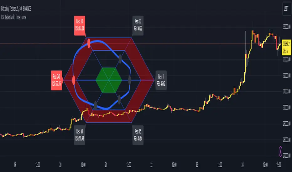
RSI Radar Multi Time FrameHello All!
First of all many Thanks to Tradingview and Pine Team for developing Pine Language all the time! Now we have a new feature and it's called Polylines and I developed RSI Radar Multi Time Frame . This script is an example and experimental work, you can use it as you wish.
The scripts gets RSI values from 6 different time frames, it doesn't matter the time frame you choose is higher/lower or chart time frame. it means that the script can get RSI values from higher or lower time frames than chart time frame.
It's designed to show RSI Radar all the time on the chart even if you zoom in/out or scroll left/right.
You can set OB/OS or RSI line colors. Also RSI polyline is shown as Curved/Hexagon optionally.
Some screenshots here:
Doesn't matter if you zoom out, it can show RSI radar in the visible area:
Another example:
You can change the colors, or see the RSI as Hexagon:
Time frames from seconds to 1Day in this example while chart time frame is any ( 30mins here )
Enjoy!
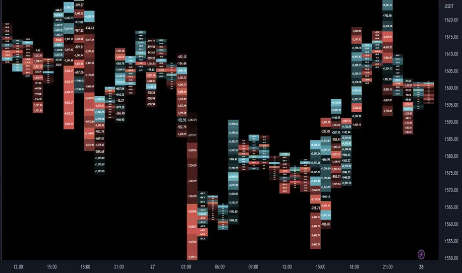
Delta Ladder [Kioseff Trading]Hello!
This script presents volume delta data in various forms!
Features
Classic mode: Volume delta boxes oriented to the right of the bar (sell closer / buy further)
On Bar mode: Volume delta boxes oriented on the bar (sell left / buy right)
Pure Ladder mode: Pure volume delta ladder
PoC highlighting
Color-coordinated delta boxes. Marginal volume differences are substantially shaded while large volume differences are lightly shaded.
Volume delta boxes can be merged and delta values removed to generate a color-only canvas reflecting vol. delta differences in price blocks.
Price bars can be split up to 497 times - allowing for greater precision.
Total volume delta for the bar and timestamp included
The image above shows Classic mode - delta blocks are oriented left/right contingent on positive/negative values!
The image above shows the same price sequence; however, delta blocks are superimposed on the price bar. Left-side blocks reflect negative delta while right-side blocks reflect positive delta! To apply this display method - select "On Bar" for the "Data Display Method" setting!
The image above shows "Pure Ladder" mode. Delta blocks remain color-coordinated; however, all delta blocks retain the same x-axis as the price bar they were calculated for!
Additionally, you can select to remove the delta values and merge the delta boxes to generate a color-based canvas indicative of volume delta at traded price levels!
The image above shows the same price sequence; however, the "Volume Assumption" setting is activated.
When active, the indicator assumes a 60/ 40 split when a level is traded at and only one metric - "buy volume" or "sell volume" is recorded. This means there shouldn't be any levels recorded where "buy volume" is greater than 0 and "sell volume" equals 0 and vice versa. While this assumption was performed arbitrarily, it may help better replicate volume delta and OI delta calculations seen on other charting platforms.
This option is configurable; you can select to have the script not assume a 60/ 40 split and instead record volume "as is" at the corresponding price level!
I plan to roll out additional features for the indicator - particularly tick-based price blocks! Stay tuned (:
Thank you!
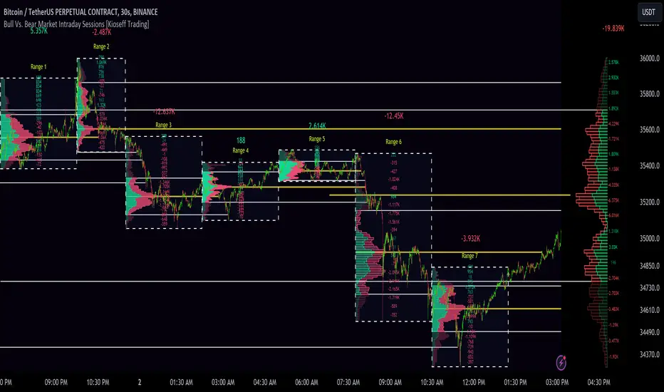
10x Bull Vs. Bear VP Intraday Sessions [Kioseff Trading]Hello!
This script "10x Bull Vs. Bear VP Intraday Sessions" lets the user configure up to 10 session ranges for Bull Vs. Bear volume profiles!
Features
Up To 10 Fixed Ranges!
Volume Profile Anchored to Fixed Range
Delta Ladder Anchored to Range
Bull vs Bear Profiles!
Standard Poc and Value Area Lines, in Addition to Separated POCs and Value Area Lines for Bull Profiles and Bear Profiles
Configurable Value Area Target
Up to 2000 Profile Rows per Visible Range
Stylistic Options for Profiles
This script generates Bull vs. Bear volume profiles for up to 10 fixed ranges!
Up to 2000 volume profile levels (price levels) Can be calculated for each profile, thanks to the new polyline feature, allowing for less aggregation / more precision of volume at price and volume delta.
Bull vs Bear Profiles
The image above shows primary functionality!
Green profiles = buying volume
Red profiles = selling volume
All colors are configurable.
Bullish & bearish POC + value areas for each fixed range are displayable!
That’s about it :D
This indicator is part of a series titled “Bull vs. Bear”.
If you have any suggestions please feel free to share!
T-Virus Sentiment [hapharmonic]🧬 T-Virus Sentiment: Visualize the Market's DNA
Remember the iconic T-Virus vial from the first Resident Evil? That powerful, swirling helix of potential has always fascinated me. It sparked an idea: what if we could visualize the market's underlying health in a similar way? What if we could capture the "genetic code" of market sentiment and contain it within a dynamic, 3D indicator? This project is the result of that idea, brought to life with Pine Script.
The indicator's main goal is to measure the strength and direction of market sentiment by analyzing the "genetic code" of price action through a variety of trusted indicators. The result is displayed as a liquid level within a DNA helix, a bubble density representing buying pressure, and a T-Virus mascot that reflects the overall mood.
🧐 Core Concept: How It Works
The primary output of the indicator is the "Active %" gauge you see on the right side of the vial. This percentage represents the overall sentiment score, calculated as an average from 7 different technical analysis tools. Each tool is analyzed on every bar and assigned a score from 1 (strong bearish pressure) to 5 (strong bullish potential).
In this indicator, we re-imagine market dynamics through the lens of a viral outbreak. A strong bear market is like a virus taking hold, pulling all technical signals down into a state of weakness. Conversely, a powerful bull market is like an antiviral serum ; positive signals rise and spread toward the top of the vial, indicating that the system is being injected with strength.
This is not just another line on a chart. It's a comprehensive sentiment dashboard designed to give an immediate, at-a-glance understanding of the confluence between 7 classic technical indicators. The incredible 3D model of the vial itself was inspired by a design concept found here .
⚛️ The 4 Core Elements of T-Virus Sentiment
These four elements work in harmony to give a complete, multi-faceted picture of market sentiment. Each component tells a different part of the story.
The Virus Mascot: An instant emotional cue. This character provides the quickest possible read on the overall market mood, combining sentiment with volume pressure.
The Antiviral Serum Level: The main quantitative output. This is the liquid level in the DNA helix and the percentage gauge on the right, representing the average sentiment score from all 7 indicators.
Buy Pressure & Bubble Density: This visualizes volume flow. The density of bubbles represents the intensity of accumulation (buying) versus distribution (selling). It's the "power" behind the move.
The Signal Distribution: This shows the confluence (or dispersion) of sentiment. Are all signals bullish and clustered at the top, or are they scattered, indicating a conflicted market? The position of the indicator labels is crucial, as each is assigned to one of five distinct zones:
Base Bottom: The market is at its weakest. Signals here suggest strong bearish control and distribution.
Lower Zone: The market is still bearish, but signals may be showing early signs of accumulation or bottoming.
Neutral Core (Center): A state of balance or sideways consolidation. The market is waiting for a new direction.
Upper Zone: Bullish momentum is becoming clear. Signals are strengthening and showing bullish control.
Top Cap: The market is "heating up" with strong bullish sentiment, potentially nearing overbought conditions.
🐂🐻 The Virus Mascot: The At-a-Glance Indicator
This character acts as a shortcut to confirm market health. It combines the sentiment score with volume, preventing false confidence in a low-volume rally.
Its state is determined by a dual-check: the overall "Antiviral Serum Level" and the "Buy Pressure" must both be above 50%.
Green & Smiling: The 'all clear' signal. This means that not only is the overall technical sentiment bullish, but it's also being supported by real buying pressure. This is a sign of a healthy bull market.
Red & Angry: A warning sign. This appears if either the sentiment is weak, or a bullish sentiment is not being confirmed by buying volume. The latter could indicate a potential "bull trap" or an exhaustive move.
This mascot can be disabled from the settings page under "Virus Mascot Styling" if a cleaner look is preferred.
🫧 Bubble Density: Gauging Buy vs. Sell Pressure
The bubbles visualize the battle between buyers and sellers. There are two modes to control how this is calculated:
Mode 1: Visible Range (The 'Big Picture' View)
This default mode is best for getting a broad, contextual understanding of the current session. It dynamically analyzes the volume of every single candlestick currently visible on the screen to calculate the buy/sell pressure ratio. It answers the question: "Over the entire period I'm looking at, who is in control?" As you zoom in or out, the calculation adapts.
Mode 2: Custom Lookback (The 'Precision' View)
This mode is for traders who need to analyze short-term pressure. You can define a fixed number of recent bars to analyze, which is perfect for scalping or understanding the volume dynamics leading into a key level. It answers the question: "What is happening right now ?" In the example above, a lookback of 2 focuses only on the most recent action, clearly showing intense, immediate selling pressure (few bubbles) and a corresponding drop in the sentiment score to 29%.
ℹ️ Interactive Tooltips: Dive Deeper
We believe in transparency, not 'black box' indicators. This feature transforms the indicator from a visual aid into an active learning tool.
Simply hover the mouse over any indicator label (like EMA, OBV, etc.) to get a detailed tooltip. It will explain the specific data points and thresholds that signal met to be placed in its current zone. This helps build trust in the signals and allows users to fine-tune the indicator settings to better match their own trading style.
🎯 The Scoring Logic Breakdown
The "Antiviral Serum Level" gauge is the average score from 7 technical analysis tools. Each is graded on a 5-point scale (1=Strong Bearish to 5=Strong Bullish). Here’s a detailed, transparent look at how each "gene" is evaluated:
Relative Strength Index (RSI)
Measures momentum and overbought/oversold conditions.
Group 1 (Strong Bearish): RSI > 80 (Extreme Overbought)
Group 2 (Bearish): 70 < RSI ≤ 80 (Overbought)
Group 3 (Neutral): 30 ≤ RSI ≤ 70
Group 4 (Bullish): 20 ≤ RSI < 30 (Oversold)
Group 5 (Strong Bullish): RSI < 20 (Extreme Oversold)
Exponential Moving Averages (EMA)
Evaluates the trend's strength and structure based on the alignment of multiple EMAs (9, 21, 50, 100, 200, 250).
Group 1 (Strong Bearish): A perfect bearish sequence (9 < 21 < 50 < ...)
Group 2 (Bearish Transition): Early signs of a potential reversal (e.g., 9 > 21 but still below 50)
Group 3 (Neutral / Mixed): MAs are intertwined or showing a partial bullish sequence.
Group 4 (Bullish): A strong bullish sequence is forming (e.g., 9 > 21 > 50 > 100)
Group 5 (Strong Bullish): A perfect bullish sequence (9 > 21 > 50 > 100 > 200 > 250)
Moving Average Convergence Divergence (MACD)
Analyzes the relationship between two moving averages to gauge momentum.
Group 1 (Strong Bearish): MACD & Histogram are negative and momentum is falling.
Group 2 (Weakening Bearish): MACD is negative but the histogram is rising or positive.
Group 3 (Neutral / Crossover): A crossover event is occurring near the zero line.
Group 4 (Bullish): MACD & Histogram are positive.
Group 5 (Strong Bullish): MACD & Histogram are positive, rising strongly, and accelerating.
Average Directional Index (ADX)
Measures trend strength, not direction. The score is based on both ADX value and the dominance of DI+ vs DI-.
Group 1 (Bearish / No Trend): ADX < 20 and DI- is dominant.
Group 2 (Developing Bearish Trend): 20 ≤ ADX < 25 and DI- is dominant.
Group 3 (Neutral / Indecision): Trend is weak or DI+ and DI- are nearly equal.
Group 4 (Developing Bullish Trend): 25 ≤ ADX ≤ 40 and DI+ is dominant.
Group 5 (Strong Bullish Trend): ADX > 40 and DI+ is dominant.
Ichimoku Cloud (IKH)
A comprehensive indicator that defines support/resistance, momentum, and trend direction.
Group 1 (Strong Bearish): Price is below the Kumo, Tenkan < Kijun, and Chikou is below price.
Group 2 (Bearish): Price is inside or below the Kumo, with mixed secondary signals.
Group 3 (Neutral / Ranging): Price is inside the Kumo, often with a Tenkan/Kijun cross.
Group 4 (Bullish): Price is above the Kumo with strong primary signals.
Group 5 (Strong Bullish): All signals are aligned bullishly: price above Kumo, bullish Tenkan/Kijun cross, bullish future Kumo, and Chikou above price.
Bollinger Bands (BB)
Measures volatility and relative price levels.
Group 1 (Strong Bearish): Price is below the lower band.
Group 2 (Bearish Territory): Price is between the lower band and the basis line.
Group 3 (Neutral): Price is hovering around the basis line.
Group 4 (Bullish Territory): Price is between the basis line and the upper band.
Group 5 (Strong Bullish): Price is above the upper band.
On-Balance Volume (OBV)
Uses volume flow to predict price changes. The score is based on OBV's trend and its position relative to its moving average.
Group 1 (Strong Bearish): OBV is below its MA and falling.
Group 2 (Weakening Bearish): OBV is below its MA but showing signs of rising.
Group 3 (Neutral): OBV is very close to its MA.
Group 4 (Bullish): OBV is above its MA and rising.
Group 5 (Strong Bullish): OBV is above its MA, rising strongly, and showing signs of a volume spike.
🧭 How to Use the T-Virus Sentiment Indicator
IMPORTANT: This indicator is a sentiment dashboard , not a direct buy/sell signal generator. Its strength lies in showing confluence and providing a quick, holistic view of the market's technical health.
Confirmation Tool: Use the "Active %" gauge to confirm a trade setup from your primary strategy. For example, if you see a bullish chart pattern, a high and rising sentiment score can add confidence to your trade.
Momentum & Trend Gauge: A consistently high score (e.g., > 75%) suggests strong, established bullish momentum. A consistently low score (< 25%) suggests strong bearish control. A score hovering around 50% often indicates a ranging or indecisive market.
Divergence & Warning System: Pay attention to divergences. If the price is making new highs but the sentiment score is failing to follow or is actively decreasing, it could be an early warning sign that the underlying momentum is weakening.
⚙️ Settings & Customization
The indicator is highly customizable to fit any trading style.
Position & Anchor: Control where the vial appears on the chart.
Styling (Vial, Helix, etc.): Nearly every visual element can be color-customized.
Signals: This is where the real power is. All underlying indicator parameters (RSI length, MACD settings, etc.) can be fine-tuned to match a personal strategy. The text labels can also be disabled if the chart feels cluttered.
Enjoy visualizing the market's DNA with the T-Virus Sentiment indicator

Intraday Spark Chart [AstrideUnicorn]The Intraday Spark Chart (ISC) is a minimalist yet powerful tool designed to track an asset’s performance relative to its daily opening price. Inspired by Nasdaq's trading-floor analog dashboards, it visualizes intraday percentage changes as a color-coded sparkline, helping traders quickly gauge momentum and session bias.
Ideal for: Day trading, scalping, and multi-asset monitoring.
Best paired with: 1m to 4H timeframes (auto-warns on higher TFs).
Key metrics:
Real-time % change from daily open.
Final daily % change (updated at session close).
Daily open price labels for orientation.
HOW TO USE
Visual Guide
Sparkline Plot:
A green area/line indicates price is above the daily open (bullish).
A red area/line signals price is below the daily open (bearish).
The baseline (0%) represents the daily open price.
Session Markers:
The dotted vertical lines separate trading days.
Gray labels near the baseline show the exact daily open price at the start of each session.
Dynamic Labels:
The labels in the upper left corner of each session range display the current (or final) daily % change. Color matches the trend (green/red) for instant readability.
Practical Use Cases
Opening Range Breakouts: Spot early momentum by observing how price reacts to the daily open.
Multi-Asset Screening: Compare intraday strength across symbols by choosing an asset in the indicator settings panel.
Session Close Prep: Anticipate daily settlement by tracking the final % change (useful for futures/swing traders).
SETTINGS
Asset (Input Symbol) : Defaults to the current chart symbol. Choose any asset to monitor its price action without switching charts - ideal for intermarket analysis or correlation tracking.

Markov Chain [3D] | FractalystWhat exactly is a Markov Chain?
This indicator uses a Markov Chain model to analyze, quantify, and visualize the transitions between market regimes (Bull, Bear, Neutral) on your chart. It dynamically detects these regimes in real-time, calculates transition probabilities, and displays them as animated 3D spheres and arrows, giving traders intuitive insight into current and future market conditions.
How does a Markov Chain work, and how should I read this spheres-and-arrows diagram?
Think of three weather modes: Sunny, Rainy, Cloudy.
Each sphere is one mode. The loop on a sphere means “stay the same next step” (e.g., Sunny again tomorrow).
The arrows leaving a sphere show where things usually go next if they change (e.g., Sunny moving to Cloudy).
Some paths matter more than others. A more prominent loop means the current mode tends to persist. A more prominent outgoing arrow means a change to that destination is the usual next step.
Direction isn’t symmetric: moving Sunny→Cloudy can behave differently than Cloudy→Sunny.
Now relabel the spheres to markets: Bull, Bear, Neutral.
Spheres: market regimes (uptrend, downtrend, range).
Self‑loop: tendency for the current regime to continue on the next bar.
Arrows: the most common next regime if a switch happens.
How to read: Start at the sphere that matches current bar state. If the loop stands out, expect continuation. If one outgoing path stands out, that switch is the typical next step. Opposite directions can differ (Bear→Neutral doesn’t have to match Neutral→Bear).
What states and transitions are shown?
The three market states visualized are:
Bullish (Bull): Upward or strong-market regime.
Bearish (Bear): Downward or weak-market regime.
Neutral: Sideways or range-bound regime.
Bidirectional animated arrows and probability labels show how likely the market is to move from one regime to another (e.g., Bull → Bear or Neutral → Bull).
How does the regime detection system work?
You can use either built-in price returns (based on adaptive Z-score normalization) or supply three custom indicators (such as volume, oscillators, etc.).
Values are statistically normalized (Z-scored) over a configurable lookback period.
The normalized outputs are classified into Bull, Bear, or Neutral zones.
If using three indicators, their regime signals are averaged and smoothed for robustness.
How are transition probabilities calculated?
On every confirmed bar, the algorithm tracks the sequence of detected market states, then builds a rolling window of transitions.
The code maintains a transition count matrix for all regime pairs (e.g., Bull → Bear).
Transition probabilities are extracted for each possible state change using Laplace smoothing for numerical stability, and frequently updated in real-time.
What is unique about the visualization?
3D animated spheres represent each regime and change visually when active.
Animated, bidirectional arrows reveal transition probabilities and allow you to see both dominant and less likely regime flows.
Particles (moving dots) animate along the arrows, enhancing the perception of regime flow direction and speed.
All elements dynamically update with each new price bar, providing a live market map in an intuitive, engaging format.
Can I use custom indicators for regime classification?
Yes! Enable the "Custom Indicators" switch and select any three chart series as inputs. These will be normalized and combined (each with equal weight), broadening the regime classification beyond just price-based movement.
What does the “Lookback Period” control?
Lookback Period (default: 100) sets how much historical data builds the probability matrix. Shorter periods adapt faster to regime changes but may be noisier. Longer periods are more stable but slower to adapt.
How is this different from a Hidden Markov Model (HMM)?
It sets the window for both regime detection and probability calculations. Lower values make the system more reactive, but potentially noisier. Higher values smooth estimates and make the system more robust.
How is this Markov Chain different from a Hidden Markov Model (HMM)?
Markov Chain (as here): All market regimes (Bull, Bear, Neutral) are directly observable on the chart. The transition matrix is built from actual detected regimes, keeping the model simple and interpretable.
Hidden Markov Model: The actual regimes are unobservable ("hidden") and must be inferred from market output or indicator "emissions" using statistical learning algorithms. HMMs are more complex, can capture more subtle structure, but are harder to visualize and require additional machine learning steps for training.
A standard Markov Chain models transitions between observable states using a simple transition matrix, while a Hidden Markov Model assumes the true states are hidden (latent) and must be inferred from observable “emissions” like price or volume data. In practical terms, a Markov Chain is transparent and easier to implement and interpret; an HMM is more expressive but requires statistical inference to estimate hidden states from data.
Markov Chain: states are observable; you directly count or estimate transition probabilities between visible states. This makes it simpler, faster, and easier to validate and tune.
HMM: states are hidden; you only observe emissions generated by those latent states. Learning involves machine learning/statistical algorithms (commonly Baum–Welch/EM for training and Viterbi for decoding) to infer both the transition dynamics and the most likely hidden state sequence from data.
How does the indicator avoid “repainting” or look-ahead bias?
All regime changes and matrix updates happen only on confirmed (closed) bars, so no future data is leaked, ensuring reliable real-time operation.
Are there practical tuning tips?
Tune the Lookback Period for your asset/timeframe: shorter for fast markets, longer for stability.
Use custom indicators if your asset has unique regime drivers.
Watch for rapid changes in transition probabilities as early warning of a possible regime shift.
Who is this indicator for?
Quants and quantitative researchers exploring probabilistic market modeling, especially those interested in regime-switching dynamics and Markov models.
Programmers and system developers who need a probabilistic regime filter for systematic and algorithmic backtesting:
The Markov Chain indicator is ideally suited for programmatic integration via its bias output (1 = Bull, 0 = Neutral, -1 = Bear).
Although the visualization is engaging, the core output is designed for automated, rules-based workflows—not for discretionary/manual trading decisions.
Developers can connect the indicator’s output directly to their Pine Script logic (using input.source()), allowing rapid and robust backtesting of regime-based strategies.
It acts as a plug-and-play regime filter: simply plug the bias output into your entry/exit logic, and you have a scientifically robust, probabilistically-derived signal for filtering, timing, position sizing, or risk regimes.
The MC's output is intentionally "trinary" (1/0/-1), focusing on clear regime states for unambiguous decision-making in code. If you require nuanced, multi-probability or soft-label state vectors, consider expanding the indicator or stacking it with a probability-weighted logic layer in your scripting.
Because it avoids subjectivity, this approach is optimal for systematic quants, algo developers building backtested, repeatable strategies based on probabilistic regime analysis.
What's the mathematical foundation behind this?
The mathematical foundation behind this Markov Chain indicator—and probabilistic regime detection in finance—draws from two principal models: the (standard) Markov Chain and the Hidden Markov Model (HMM).
How to use this indicator programmatically?
The Markov Chain indicator automatically exports a bias value (+1 for Bullish, -1 for Bearish, 0 for Neutral) as a plot visible in the Data Window. This allows you to integrate its regime signal into your own scripts and strategies for backtesting, automation, or live trading.
Step-by-Step Integration with Pine Script (input.source)
Add the Markov Chain indicator to your chart.
This must be done first, since your custom script will "pull" the bias signal from the indicator's plot.
In your strategy, create an input using input.source()
Example:
//@version=5
strategy("MC Bias Strategy Example")
mcBias = input.source(close, "MC Bias Source")
After saving, go to your script’s settings. For the “MC Bias Source” input, select the plot/output of the Markov Chain indicator (typically its bias plot).
Use the bias in your trading logic
Example (long only on Bull, flat otherwise):
if mcBias == 1
strategy.entry("Long", strategy.long)
else
strategy.close("Long")
For more advanced workflows, combine mcBias with additional filters or trailing stops.
How does this work behind-the-scenes?
TradingView’s input.source() lets you use any plot from another indicator as a real-time, “live” data feed in your own script (source).
The selected bias signal is available to your Pine code as a variable, enabling logical decisions based on regime (trend-following, mean-reversion, etc.).
This enables powerful strategy modularity : decouple regime detection from entry/exit logic, allowing fast experimentation without rewriting core signal code.
Integrating 45+ Indicators with Your Markov Chain — How & Why
The Enhanced Custom Indicators Export script exports a massive suite of over 45 technical indicators—ranging from classic momentum (RSI, MACD, Stochastic, etc.) to trend, volume, volatility, and oscillator tools—all pre-calculated, centered/scaled, and available as plots.
// Enhanced Custom Indicators Export - 45 Technical Indicators
// Comprehensive technical analysis suite for advanced market regime detection
//@version=6
indicator('Enhanced Custom Indicators Export | Fractalyst', shorttitle='Enhanced CI Export', overlay=false, scale=scale.right, max_labels_count=500, max_lines_count=500)
// |----- Input Parameters -----| //
momentum_group = "Momentum Indicators"
trend_group = "Trend Indicators"
volume_group = "Volume Indicators"
volatility_group = "Volatility Indicators"
oscillator_group = "Oscillator Indicators"
display_group = "Display Settings"
// Common lengths
length_14 = input.int(14, "Standard Length (14)", minval=1, maxval=100, group=momentum_group)
length_20 = input.int(20, "Medium Length (20)", minval=1, maxval=200, group=trend_group)
length_50 = input.int(50, "Long Length (50)", minval=1, maxval=200, group=trend_group)
// Display options
show_table = input.bool(true, "Show Values Table", group=display_group)
table_size = input.string("Small", "Table Size", options= , group=display_group)
// |----- MOMENTUM INDICATORS (15 indicators) -----| //
// 1. RSI (Relative Strength Index)
rsi_14 = ta.rsi(close, length_14)
rsi_centered = rsi_14 - 50
// 2. Stochastic Oscillator
stoch_k = ta.stoch(close, high, low, length_14)
stoch_d = ta.sma(stoch_k, 3)
stoch_centered = stoch_k - 50
// 3. Williams %R
williams_r = ta.stoch(close, high, low, length_14) - 100
// 4. MACD (Moving Average Convergence Divergence)
= ta.macd(close, 12, 26, 9)
// 5. Momentum (Rate of Change)
momentum = ta.mom(close, length_14)
momentum_pct = (momentum / close ) * 100
// 6. Rate of Change (ROC)
roc = ta.roc(close, length_14)
// 7. Commodity Channel Index (CCI)
cci = ta.cci(close, length_20)
// 8. Money Flow Index (MFI)
mfi = ta.mfi(close, length_14)
mfi_centered = mfi - 50
// 9. Awesome Oscillator (AO)
ao = ta.sma(hl2, 5) - ta.sma(hl2, 34)
// 10. Accelerator Oscillator (AC)
ac = ao - ta.sma(ao, 5)
// 11. Chande Momentum Oscillator (CMO)
cmo = ta.cmo(close, length_14)
// 12. Detrended Price Oscillator (DPO)
dpo = close - ta.sma(close, length_20)
// 13. Price Oscillator (PPO)
ppo = ta.sma(close, 12) - ta.sma(close, 26)
ppo_pct = (ppo / ta.sma(close, 26)) * 100
// 14. TRIX
trix_ema1 = ta.ema(close, length_14)
trix_ema2 = ta.ema(trix_ema1, length_14)
trix_ema3 = ta.ema(trix_ema2, length_14)
trix = ta.roc(trix_ema3, 1) * 10000
// 15. Klinger Oscillator
klinger = ta.ema(volume * (high + low + close) / 3, 34) - ta.ema(volume * (high + low + close) / 3, 55)
// 16. Fisher Transform
fisher_hl2 = 0.5 * (hl2 - ta.lowest(hl2, 10)) / (ta.highest(hl2, 10) - ta.lowest(hl2, 10)) - 0.25
fisher = 0.5 * math.log((1 + fisher_hl2) / (1 - fisher_hl2))
// 17. Stochastic RSI
stoch_rsi = ta.stoch(rsi_14, rsi_14, rsi_14, length_14)
stoch_rsi_centered = stoch_rsi - 50
// 18. Relative Vigor Index (RVI)
rvi_num = ta.swma(close - open)
rvi_den = ta.swma(high - low)
rvi = rvi_den != 0 ? rvi_num / rvi_den : 0
// 19. Balance of Power (BOP)
bop = (close - open) / (high - low)
// |----- TREND INDICATORS (10 indicators) -----| //
// 20. Simple Moving Average Momentum
sma_20 = ta.sma(close, length_20)
sma_momentum = ((close - sma_20) / sma_20) * 100
// 21. Exponential Moving Average Momentum
ema_20 = ta.ema(close, length_20)
ema_momentum = ((close - ema_20) / ema_20) * 100
// 22. Parabolic SAR
sar = ta.sar(0.02, 0.02, 0.2)
sar_trend = close > sar ? 1 : -1
// 23. Linear Regression Slope
lr_slope = ta.linreg(close, length_20, 0) - ta.linreg(close, length_20, 1)
// 24. Moving Average Convergence (MAC)
mac = ta.sma(close, 10) - ta.sma(close, 30)
// 25. Trend Intensity Index (TII)
tii_sum = 0.0
for i = 1 to length_20
tii_sum += close > close ? 1 : 0
tii = (tii_sum / length_20) * 100
// 26. Ichimoku Cloud Components
ichimoku_tenkan = (ta.highest(high, 9) + ta.lowest(low, 9)) / 2
ichimoku_kijun = (ta.highest(high, 26) + ta.lowest(low, 26)) / 2
ichimoku_signal = ichimoku_tenkan > ichimoku_kijun ? 1 : -1
// 27. MESA Adaptive Moving Average (MAMA)
mama_alpha = 2.0 / (length_20 + 1)
mama = ta.ema(close, length_20)
mama_momentum = ((close - mama) / mama) * 100
// 28. Zero Lag Exponential Moving Average (ZLEMA)
zlema_lag = math.round((length_20 - 1) / 2)
zlema_data = close + (close - close )
zlema = ta.ema(zlema_data, length_20)
zlema_momentum = ((close - zlema) / zlema) * 100
// |----- VOLUME INDICATORS (6 indicators) -----| //
// 29. On-Balance Volume (OBV)
obv = ta.obv
// 30. Volume Rate of Change (VROC)
vroc = ta.roc(volume, length_14)
// 31. Price Volume Trend (PVT)
pvt = ta.pvt
// 32. Negative Volume Index (NVI)
nvi = 0.0
nvi := volume < volume ? nvi + ((close - close ) / close ) * nvi : nvi
// 33. Positive Volume Index (PVI)
pvi = 0.0
pvi := volume > volume ? pvi + ((close - close ) / close ) * pvi : pvi
// 34. Volume Oscillator
vol_osc = ta.sma(volume, 5) - ta.sma(volume, 10)
// 35. Ease of Movement (EOM)
eom_distance = high - low
eom_box_height = volume / 1000000
eom = eom_box_height != 0 ? eom_distance / eom_box_height : 0
eom_sma = ta.sma(eom, length_14)
// 36. Force Index
force_index = volume * (close - close )
force_index_sma = ta.sma(force_index, length_14)
// |----- VOLATILITY INDICATORS (10 indicators) -----| //
// 37. Average True Range (ATR)
atr = ta.atr(length_14)
atr_pct = (atr / close) * 100
// 38. Bollinger Bands Position
bb_basis = ta.sma(close, length_20)
bb_dev = 2.0 * ta.stdev(close, length_20)
bb_upper = bb_basis + bb_dev
bb_lower = bb_basis - bb_dev
bb_position = bb_dev != 0 ? (close - bb_basis) / bb_dev : 0
bb_width = bb_dev != 0 ? (bb_upper - bb_lower) / bb_basis * 100 : 0
// 39. Keltner Channels Position
kc_basis = ta.ema(close, length_20)
kc_range = ta.ema(ta.tr, length_20)
kc_upper = kc_basis + (2.0 * kc_range)
kc_lower = kc_basis - (2.0 * kc_range)
kc_position = kc_range != 0 ? (close - kc_basis) / kc_range : 0
// 40. Donchian Channels Position
dc_upper = ta.highest(high, length_20)
dc_lower = ta.lowest(low, length_20)
dc_basis = (dc_upper + dc_lower) / 2
dc_position = (dc_upper - dc_lower) != 0 ? (close - dc_basis) / (dc_upper - dc_lower) : 0
// 41. Standard Deviation
std_dev = ta.stdev(close, length_20)
std_dev_pct = (std_dev / close) * 100
// 42. Relative Volatility Index (RVI)
rvi_up = ta.stdev(close > close ? close : 0, length_14)
rvi_down = ta.stdev(close < close ? close : 0, length_14)
rvi_total = rvi_up + rvi_down
rvi_volatility = rvi_total != 0 ? (rvi_up / rvi_total) * 100 : 50
// 43. Historical Volatility
hv_returns = math.log(close / close )
hv = ta.stdev(hv_returns, length_20) * math.sqrt(252) * 100
// 44. Garman-Klass Volatility
gk_vol = math.log(high/low) * math.log(high/low) - (2*math.log(2)-1) * math.log(close/open) * math.log(close/open)
gk_volatility = math.sqrt(ta.sma(gk_vol, length_20)) * 100
// 45. Parkinson Volatility
park_vol = math.log(high/low) * math.log(high/low)
parkinson = math.sqrt(ta.sma(park_vol, length_20) / (4 * math.log(2))) * 100
// 46. Rogers-Satchell Volatility
rs_vol = math.log(high/close) * math.log(high/open) + math.log(low/close) * math.log(low/open)
rogers_satchell = math.sqrt(ta.sma(rs_vol, length_20)) * 100
// |----- OSCILLATOR INDICATORS (5 indicators) -----| //
// 47. Elder Ray Index
elder_bull = high - ta.ema(close, 13)
elder_bear = low - ta.ema(close, 13)
elder_power = elder_bull + elder_bear
// 48. Schaff Trend Cycle (STC)
stc_macd = ta.ema(close, 23) - ta.ema(close, 50)
stc_k = ta.stoch(stc_macd, stc_macd, stc_macd, 10)
stc_d = ta.ema(stc_k, 3)
stc = ta.stoch(stc_d, stc_d, stc_d, 10)
// 49. Coppock Curve
coppock_roc1 = ta.roc(close, 14)
coppock_roc2 = ta.roc(close, 11)
coppock = ta.wma(coppock_roc1 + coppock_roc2, 10)
// 50. Know Sure Thing (KST)
kst_roc1 = ta.roc(close, 10)
kst_roc2 = ta.roc(close, 15)
kst_roc3 = ta.roc(close, 20)
kst_roc4 = ta.roc(close, 30)
kst = ta.sma(kst_roc1, 10) + 2*ta.sma(kst_roc2, 10) + 3*ta.sma(kst_roc3, 10) + 4*ta.sma(kst_roc4, 15)
// 51. Percentage Price Oscillator (PPO)
ppo_line = ((ta.ema(close, 12) - ta.ema(close, 26)) / ta.ema(close, 26)) * 100
ppo_signal = ta.ema(ppo_line, 9)
ppo_histogram = ppo_line - ppo_signal
// |----- PLOT MAIN INDICATORS -----| //
// Plot key momentum indicators
plot(rsi_centered, title="01_RSI_Centered", color=color.purple, linewidth=1)
plot(stoch_centered, title="02_Stoch_Centered", color=color.blue, linewidth=1)
plot(williams_r, title="03_Williams_R", color=color.red, linewidth=1)
plot(macd_histogram, title="04_MACD_Histogram", color=color.orange, linewidth=1)
plot(cci, title="05_CCI", color=color.green, linewidth=1)
// Plot trend indicators
plot(sma_momentum, title="06_SMA_Momentum", color=color.navy, linewidth=1)
plot(ema_momentum, title="07_EMA_Momentum", color=color.maroon, linewidth=1)
plot(sar_trend, title="08_SAR_Trend", color=color.teal, linewidth=1)
plot(lr_slope, title="09_LR_Slope", color=color.lime, linewidth=1)
plot(mac, title="10_MAC", color=color.fuchsia, linewidth=1)
// Plot volatility indicators
plot(atr_pct, title="11_ATR_Pct", color=color.yellow, linewidth=1)
plot(bb_position, title="12_BB_Position", color=color.aqua, linewidth=1)
plot(kc_position, title="13_KC_Position", color=color.olive, linewidth=1)
plot(std_dev_pct, title="14_StdDev_Pct", color=color.silver, linewidth=1)
plot(bb_width, title="15_BB_Width", color=color.gray, linewidth=1)
// Plot volume indicators
plot(vroc, title="16_VROC", color=color.blue, linewidth=1)
plot(eom_sma, title="17_EOM", color=color.red, linewidth=1)
plot(vol_osc, title="18_Vol_Osc", color=color.green, linewidth=1)
plot(force_index_sma, title="19_Force_Index", color=color.orange, linewidth=1)
plot(obv, title="20_OBV", color=color.purple, linewidth=1)
// Plot additional oscillators
plot(ao, title="21_Awesome_Osc", color=color.navy, linewidth=1)
plot(cmo, title="22_CMO", color=color.maroon, linewidth=1)
plot(dpo, title="23_DPO", color=color.teal, linewidth=1)
plot(trix, title="24_TRIX", color=color.lime, linewidth=1)
plot(fisher, title="25_Fisher", color=color.fuchsia, linewidth=1)
// Plot more momentum indicators
plot(mfi_centered, title="26_MFI_Centered", color=color.yellow, linewidth=1)
plot(ac, title="27_AC", color=color.aqua, linewidth=1)
plot(ppo_pct, title="28_PPO_Pct", color=color.olive, linewidth=1)
plot(stoch_rsi_centered, title="29_StochRSI_Centered", color=color.silver, linewidth=1)
plot(klinger, title="30_Klinger", color=color.gray, linewidth=1)
// Plot trend continuation
plot(tii, title="31_TII", color=color.blue, linewidth=1)
plot(ichimoku_signal, title="32_Ichimoku_Signal", color=color.red, linewidth=1)
plot(mama_momentum, title="33_MAMA_Momentum", color=color.green, linewidth=1)
plot(zlema_momentum, title="34_ZLEMA_Momentum", color=color.orange, linewidth=1)
plot(bop, title="35_BOP", color=color.purple, linewidth=1)
// Plot volume continuation
plot(nvi, title="36_NVI", color=color.navy, linewidth=1)
plot(pvi, title="37_PVI", color=color.maroon, linewidth=1)
plot(momentum_pct, title="38_Momentum_Pct", color=color.teal, linewidth=1)
plot(roc, title="39_ROC", color=color.lime, linewidth=1)
plot(rvi, title="40_RVI", color=color.fuchsia, linewidth=1)
// Plot volatility continuation
plot(dc_position, title="41_DC_Position", color=color.yellow, linewidth=1)
plot(rvi_volatility, title="42_RVI_Volatility", color=color.aqua, linewidth=1)
plot(hv, title="43_Historical_Vol", color=color.olive, linewidth=1)
plot(gk_volatility, title="44_GK_Volatility", color=color.silver, linewidth=1)
plot(parkinson, title="45_Parkinson_Vol", color=color.gray, linewidth=1)
// Plot final oscillators
plot(rogers_satchell, title="46_RS_Volatility", color=color.blue, linewidth=1)
plot(elder_power, title="47_Elder_Power", color=color.red, linewidth=1)
plot(stc, title="48_STC", color=color.green, linewidth=1)
plot(coppock, title="49_Coppock", color=color.orange, linewidth=1)
plot(kst, title="50_KST", color=color.purple, linewidth=1)
// Plot final indicators
plot(ppo_histogram, title="51_PPO_Histogram", color=color.navy, linewidth=1)
plot(pvt, title="52_PVT", color=color.maroon, linewidth=1)
// |----- Reference Lines -----| //
hline(0, "Zero Line", color=color.gray, linestyle=hline.style_dashed, linewidth=1)
hline(50, "Midline", color=color.gray, linestyle=hline.style_dotted, linewidth=1)
hline(-50, "Lower Midline", color=color.gray, linestyle=hline.style_dotted, linewidth=1)
hline(25, "Upper Threshold", color=color.gray, linestyle=hline.style_dotted, linewidth=1)
hline(-25, "Lower Threshold", color=color.gray, linestyle=hline.style_dotted, linewidth=1)
// |----- Enhanced Information Table -----| //
if show_table and barstate.islast
table_position = position.top_right
table_text_size = table_size == "Tiny" ? size.tiny : table_size == "Small" ? size.small : size.normal
var table info_table = table.new(table_position, 3, 18, bgcolor=color.new(color.white, 85), border_width=1, border_color=color.gray)
// Headers
table.cell(info_table, 0, 0, 'Category', text_color=color.black, text_size=table_text_size, bgcolor=color.new(color.blue, 70))
table.cell(info_table, 1, 0, 'Indicator', text_color=color.black, text_size=table_text_size, bgcolor=color.new(color.blue, 70))
table.cell(info_table, 2, 0, 'Value', text_color=color.black, text_size=table_text_size, bgcolor=color.new(color.blue, 70))
// Key Momentum Indicators
table.cell(info_table, 0, 1, 'MOMENTUM', text_color=color.purple, text_size=table_text_size, bgcolor=color.new(color.purple, 90))
table.cell(info_table, 1, 1, 'RSI Centered', text_color=color.purple, text_size=table_text_size)
table.cell(info_table, 2, 1, str.tostring(rsi_centered, '0.00'), text_color=color.purple, text_size=table_text_size)
table.cell(info_table, 0, 2, '', text_color=color.blue, text_size=table_text_size)
table.cell(info_table, 1, 2, 'Stoch Centered', text_color=color.blue, text_size=table_text_size)
table.cell(info_table, 2, 2, str.tostring(stoch_centered, '0.00'), text_color=color.blue, text_size=table_text_size)
table.cell(info_table, 0, 3, '', text_color=color.red, text_size=table_text_size)
table.cell(info_table, 1, 3, 'Williams %R', text_color=color.red, text_size=table_text_size)
table.cell(info_table, 2, 3, str.tostring(williams_r, '0.00'), text_color=color.red, text_size=table_text_size)
table.cell(info_table, 0, 4, '', text_color=color.orange, text_size=table_text_size)
table.cell(info_table, 1, 4, 'MACD Histogram', text_color=color.orange, text_size=table_text_size)
table.cell(info_table, 2, 4, str.tostring(macd_histogram, '0.000'), text_color=color.orange, text_size=table_text_size)
table.cell(info_table, 0, 5, '', text_color=color.green, text_size=table_text_size)
table.cell(info_table, 1, 5, 'CCI', text_color=color.green, text_size=table_text_size)
table.cell(info_table, 2, 5, str.tostring(cci, '0.00'), text_color=color.green, text_size=table_text_size)
// Key Trend Indicators
table.cell(info_table, 0, 6, 'TREND', text_color=color.navy, text_size=table_text_size, bgcolor=color.new(color.navy, 90))
table.cell(info_table, 1, 6, 'SMA Momentum %', text_color=color.navy, text_size=table_text_size)
table.cell(info_table, 2, 6, str.tostring(sma_momentum, '0.00'), text_color=color.navy, text_size=table_text_size)
table.cell(info_table, 0, 7, '', text_color=color.maroon, text_size=table_text_size)
table.cell(info_table, 1, 7, 'EMA Momentum %', text_color=color.maroon, text_size=table_text_size)
table.cell(info_table, 2, 7, str.tostring(ema_momentum, '0.00'), text_color=color.maroon, text_size=table_text_size)
table.cell(info_table, 0, 8, '', text_color=color.teal, text_size=table_text_size)
table.cell(info_table, 1, 8, 'SAR Trend', text_color=color.teal, text_size=table_text_size)
table.cell(info_table, 2, 8, str.tostring(sar_trend, '0'), text_color=color.teal, text_size=table_text_size)
table.cell(info_table, 0, 9, '', text_color=color.lime, text_size=table_text_size)
table.cell(info_table, 1, 9, 'Linear Regression', text_color=color.lime, text_size=table_text_size)
table.cell(info_table, 2, 9, str.tostring(lr_slope, '0.000'), text_color=color.lime, text_size=table_text_size)
// Key Volatility Indicators
table.cell(info_table, 0, 10, 'VOLATILITY', text_color=color.yellow, text_size=table_text_size, bgcolor=color.new(color.yellow, 90))
table.cell(info_table, 1, 10, 'ATR %', text_color=color.yellow, text_size=table_text_size)
table.cell(info_table, 2, 10, str.tostring(atr_pct, '0.00'), text_color=color.yellow, text_size=table_text_size)
table.cell(info_table, 0, 11, '', text_color=color.aqua, text_size=table_text_size)
table.cell(info_table, 1, 11, 'BB Position', text_color=color.aqua, text_size=table_text_size)
table.cell(info_table, 2, 11, str.tostring(bb_position, '0.00'), text_color=color.aqua, text_size=table_text_size)
table.cell(info_table, 0, 12, '', text_color=color.olive, text_size=table_text_size)
table.cell(info_table, 1, 12, 'KC Position', text_color=color.olive, text_size=table_text_size)
table.cell(info_table, 2, 12, str.tostring(kc_position, '0.00'), text_color=color.olive, text_size=table_text_size)
// Key Volume Indicators
table.cell(info_table, 0, 13, 'VOLUME', text_color=color.blue, text_size=table_text_size, bgcolor=color.new(color.blue, 90))
table.cell(info_table, 1, 13, 'Volume ROC', text_color=color.blue, text_size=table_text_size)
table.cell(info_table, 2, 13, str.tostring(vroc, '0.00'), text_color=color.blue, text_size=table_text_size)
table.cell(info_table, 0, 14, '', text_color=color.red, text_size=table_text_size)
table.cell(info_table, 1, 14, 'EOM', text_color=color.red, text_size=table_text_size)
table.cell(info_table, 2, 14, str.tostring(eom_sma, '0.000'), text_color=color.red, text_size=table_text_size)
// Key Oscillators
table.cell(info_table, 0, 15, 'OSCILLATORS', text_color=color.purple, text_size=table_text_size, bgcolor=color.new(color.purple, 90))
table.cell(info_table, 1, 15, 'Awesome Osc', text_color=color.blue, text_size=table_text_size)
table.cell(info_table, 2, 15, str.tostring(ao, '0.000'), text_color=color.blue, text_size=table_text_size)
table.cell(info_table, 0, 16, '', text_color=color.red, text_size=table_text_size)
table.cell(info_table, 1, 16, 'Fisher Transform', text_color=color.red, text_size=table_text_size)
table.cell(info_table, 2, 16, str.tostring(fisher, '0.000'), text_color=color.red, text_size=table_text_size)
// Summary Statistics
table.cell(info_table, 0, 17, 'SUMMARY', text_color=color.black, text_size=table_text_size, bgcolor=color.new(color.gray, 70))
table.cell(info_table, 1, 17, 'Total Indicators: 52', text_color=color.black, text_size=table_text_size)
regime_color = rsi_centered > 10 ? color.green : rsi_centered < -10 ? color.red : color.gray
regime_text = rsi_centered > 10 ? "BULLISH" : rsi_centered < -10 ? "BEARISH" : "NEUTRAL"
table.cell(info_table, 2, 17, regime_text, text_color=regime_color, text_size=table_text_size)
This makes it the perfect “indicator backbone” for quantitative and systematic traders who want to prototype, combine, and test new regime detection models—especially in combination with the Markov Chain indicator.
How to use this script with the Markov Chain for research and backtesting:
Add the Enhanced Indicator Export to your chart.
Every calculated indicator is available as an individual data stream.
Connect the indicator(s) you want as custom input(s) to the Markov Chain’s “Custom Indicators” option.
In the Markov Chain indicator’s settings, turn ON the custom indicator mode.
For each of the three custom indicator inputs, select the exported plot from the Enhanced Export script—the menu lists all 45+ signals by name.
This creates a powerful, modular regime-detection engine where you can mix-and-match momentum, trend, volume, or custom combinations for advanced filtering.
Backtest regime logic directly.
Once you’ve connected your chosen indicators, the Markov Chain script performs regime detection (Bull/Neutral/Bear) based on your selected features—not just price returns.
The regime detection is robust, automatically normalized (using Z-score), and outputs bias (1, -1, 0) for plug-and-play integration.
Export the regime bias for programmatic use.
As described above, use input.source() in your Pine Script strategy or system and link the bias output.
You can now filter signals, control trade direction/size, or design pairs-trading that respect true, indicator-driven market regimes.
With this framework, you’re not limited to static or simplistic regime filters. You can rigorously define, test, and refine what “market regime” means for your strategies—using the technical features that matter most to you.
Optimize your signal generation by backtesting across a universe of meaningful indicator blends.
Enhance risk management with objective, real-time regime boundaries.
Accelerate your research: iterate quickly, swap indicator components, and see results with minimal code changes.
Automate multi-asset or pairs-trading by integrating regime context directly into strategy logic.
Add both scripts to your chart, connect your preferred features, and start investigating your best regime-based trades—entirely within the TradingView ecosystem.
References & Further Reading
Ang, A., & Bekaert, G. (2002). “Regime Switches in Interest Rates.” Journal of Business & Economic Statistics, 20(2), 163–182.
Hamilton, J. D. (1989). “A New Approach to the Economic Analysis of Nonstationary Time Series and the Business Cycle.” Econometrica, 57(2), 357–384.
Markov, A. A. (1906). "Extension of the Limit Theorems of Probability Theory to a Sum of Variables Connected in a Chain." The Notes of the Imperial Academy of Sciences of St. Petersburg.
Guidolin, M., & Timmermann, A. (2007). “Asset Allocation under Multivariate Regime Switching.” Journal of Economic Dynamics and Control, 31(11), 3503–3544.
Murphy, J. J. (1999). Technical Analysis of the Financial Markets. New York Institute of Finance.
Brock, W., Lakonishok, J., & LeBaron, B. (1992). “Simple Technical Trading Rules and the Stochastic Properties of Stock Returns.” Journal of Finance, 47(5), 1731–1764.
Zucchini, W., MacDonald, I. L., & Langrock, R. (2017). Hidden Markov Models for Time Series: An Introduction Using R (2nd ed.). Chapman and Hall/CRC.
On Quantitative Finance and Markov Models:
Lo, A. W., & Hasanhodzic, J. (2009). The Heretics of Finance: Conversations with Leading Practitioners of Technical Analysis. Bloomberg Press.
Patterson, S. (2016). The Man Who Solved the Market: How Jim Simons Launched the Quant Revolution. Penguin Press.
TradingView Pine Script Documentation: www.tradingview.com
TradingView Blog: “Use an Input From Another Indicator With Your Strategy” www.tradingview.com
GeeksforGeeks: “What is the Difference Between Markov Chains and Hidden Markov Models?” www.geeksforgeeks.org
What makes this indicator original and unique?
- On‑chart, real‑time Markov. The chain is drawn directly on your chart. You see the current regime, its tendency to stay (self‑loop), and the usual next step (arrows) as bars confirm.
- Source‑agnostic by design. The engine runs on any series you select via input.source() — price, your own oscillator, a composite score, anything you compute in the script.
- Automatic normalization + regime mapping. Different inputs live on different scales. The script standardizes your chosen source and maps it into clear regimes (e.g., Bull / Bear / Neutral) without you micromanaging thresholds each time.
- Rolling, bar‑by‑bar learning. Transition tendencies are computed from a rolling window of confirmed bars. What you see is exactly what the market did in that window.
- Fast experimentation. Switch the source, adjust the window, and the Markov view updates instantly. It’s a rapid way to test ideas and feel regime persistence/switch behavior.
Integrate your own signals (using input.source())
- In settings, choose the Source . This is powered by input.source() .
- Feed it price, an indicator you compute inside the script, or a custom composite series.
- The script will automatically normalize that series and process it through the Markov engine, mapping it to regimes and updating the on‑chart spheres/arrows in real time.
Credits:
Deep gratitude to @RicardoSantos for both the foundational Markov chain processing engine and inspiring open-source contributions, which made advanced probabilistic market modeling accessible to the TradingView community.
Special thanks to @Alien_Algorithms for the innovative and visually stunning 3D sphere logic that powers the indicator’s animated, regime-based visualization.
Disclaimer
This tool summarizes recent behavior. It is not financial advice and not a guarantee of future results.

Correlation HeatMap [TradingFinder] Sessions Data Science Stats🔵 Introduction
n financial markets, correlation describes the statistical relationship between the price movements of two assets and how they interact over time. It plays a key role in both trading and investing by helping analyze asset behavior, manage portfolio risk, and understand intermarket dynamics. The Correlation Heatmap is a visual tool that shows how the correlation between multiple assets and a central reference asset (the Main Symbol) changes over time.
It supports four market types forex, stocks, crypto, and a custom mode making it adaptable to different trading environments. The heatmap uses a color-coded grid where warmer tones represent stronger negative correlations and cooler tones indicate stronger positive ones. This intuitive color system allows traders to quickly identify when assets move together or diverge, offering real-time insights that go beyond traditional correlation tables.
🟣 How to Interpret the Heatmap Visually ?
Each cell represents the correlation between the main symbol and one compared asset at a specific time.
Warm colors (e.g. red, orange) suggest strong negative correlation as one asset rises, the other tends to fall.
Cool colors (e.g. blue, green) suggest strong positive correlation both assets tend to move in the same direction.
Lighter shades indicate weaker correlations, while darker shades indicate stronger correlations.
The heatmap updates over time, allowing users to detect changes in correlation during market events or trading sessions.
One of the standout features of this indicator is its ability to overlay global market sessions such as Tokyo, London, New York, or major equity opens directly onto the heatmap timeline. This alignment lets traders observe how correlation structures respond to real-world session changes. For example, they can spot when assets shift from being inversely correlated to moving together as a new session opens, potentially signaling new momentum or macro flow. The customizable symbol setup (including up to 20 compared assets) makes it ideal not only for forex and crypto traders but also for multi-asset and sector-based stock analysis.
🟣 Use Cases and Advantages
Analyze sector rotation in equities by tracking correlation to major indices like SPX or DJI.
Monitor altcoin behavior relative to Bitcoin to find early entry opportunities in crypto markets.
Detect changes in currency alignment with DXY across trading sessions in forex.
Identify correlation breakdowns during market volatility, signaling possible new trends.
Use correlation shifts as confirmation for trade setups or to hedge multi-asset exposure
🔵 How to Use
Correlation is one of the core concepts in financial analysis and allows traders to understand how assets behave in relation to one another. The Correlation Heatmap extends this idea by going beyond a simple number or static matrix. Instead, it presents a dynamic visual map of how correlations shift over time.
In this indicator, a Main Symbol is selected as the reference point for analysis. In standard modes such as forex, stocks, or crypto, the symbol currently shown on the main chart is automatically used as the main symbol. This allows users to begin correlation analysis right away without adjusting any settings.
The horizontal axis of the heatmap shows time, while the vertical axis lists the selected assets. Each cell on the heatmap shows the correlation between that asset and the main symbol at a given moment.
This approach is especially useful for intermarket analysis. In forex, for example, tracking how currency pairs like OANDA:EURUSD EURUSD, FX:GBPUSD GBPUSD, and PEPPERSTONE:AUDUSD AUDUSD correlate with TVC:DXY DXY can give insight into broader capital flow.
If these pairs start showing increasing positive correlation with DXY say, shifting from blue to light green it could signal the start of a new phase or reversal. Conversely, if negative correlation fades gradually, it may suggest weakening relationships and more independent or volatile movement.
In the crypto market, watching how altcoins correlate with Bitcoin can help identify ideal entry points in secondary assets. In the stock market, analyzing how companies within the same sector move in relation to a major index like SP:SPX SPX or DJ:DJI DJI is also a highly effective technique for both technical and fundamental analysts.
This indicator not only visualizes correlation but also displays major market sessions. When enabled, this feature helps traders observe how correlation behavior changes at the start of each session, whether it's Tokyo, London, New York, or the opening of stock exchanges. Many key shifts, breakouts, or reversals tend to happen around these times, and the heatmap makes them easy to spot.
Another important feature is the market selection mode. Users can switch between forex, crypto, stocks, or custom markets and see correlation behavior specific to each one. In custom mode, users can manually select any combination of symbols for more advanced or personalized analysis. This makes the heatmap valuable not only for forex traders but also for stock traders, crypto analysts, and multi-asset strategists.
Finally, the heatmap's color-coded design helps users make sense of the data quickly. Warm colors such as red and orange reflect stronger negative correlations, while cool colors like blue and green represent stronger positive relationships. This simplicity and clarity make the tool accessible to both beginners and experienced traders.
🔵 Settings
Correlation Period: Allows you to set how many historical bars are used for calculating correlation. A higher number means a smoother, slower-moving heatmap, while a lower number makes it more responsive to recent changes.
Select Market: Lets you choose between Forex, Stock, Crypto, or Custom. In the first three options, the chart’s active symbol is automatically used as the Main Symbol. In Custom mode, you can manually define the Main Symbol and up to 20 Compared Symbols.
Show Open Session: Enables the display of major trading sessions such as Tokyo, London, New York, or equity market opening hours directly on the timeline. This helps you connect correlation shifts with real-world market activity.
Market Mode: Lets you select whether the displayed sessions relate to the forex or stock market.
🔵 Conclusion
The Correlation Heatmap is a robust and flexible tool for analyzing the relationship between assets across different markets. By tracking how correlations change in real time, traders can better identify alignment or divergence between symbols and gain valuable insights into market structure.
Support for multiple asset classes, session overlays, and intuitive visual cues make this one of the most effective tools for intermarket analysis.
Whether you’re looking to manage portfolio risk, validate entry points, or simply understand capital flow across markets, this heatmap provides a clear and actionable perspective that you can rely on.

Volume Rotor Clock [hapharmonic]🕰️ Volume Rotor Clock
The Volume Rotor Clock is an indicator that separates buy and sell volume, compiling these volumes over a recent number of bars or a specified past period, as defined by the user. This helps to reveal accumulation (buying) or distribution (selling) behavior, showing which side has superior volume. With its unique and beautiful display, the Volume Rotor Clock is more than just a timepiece; it's a dynamic dashboard that visualizes the buying and selling pressure of your favorite symbols, all wrapped in an elegant and fully customizable interface.
Instead of just tracking price, this indicator focuses on the engine behind the movement: volume. It helps you instantly identify which assets are under accumulation (buying) and which are under distribution (selling).
---
🎨 20 Pre-configured Templates
---
🧐 Interpreting the Clock Display
The interface is designed to give you multiple layers of information at a glance. Let's break down what each part represents.
1. The Main Clock Hands (Current Chart Symbol)
The clock hands—hour, minute, and second—are dedicated to the symbol on your current active chart .
Minute Hand: Displays the base currency of the current symbol (e.g., USDT, USD) at its tip.
Hour Hand: Displays the percentage of the winning volume side (buy vs. sell) at its tip.
Color Gauge: The color of the text characters at the tip of both the hour and minute hands acts as your primary volume gauge for the current symbol.
If buy volume is dominant , the text will be green .
If sell volume is dominant , the text will be red .
Tooltip: Hovering your mouse over the text at the tip of the hour or minute or other spherical elements hand will reveal a detailed tooltip with the precise Buy Volume, Sell Volume, Total Volume, Buy %, and Sell % for the current chart's symbol.
2. The Volume Scanner: Bulls & Bears (Symbols Inside the Clock) 🐂🐻
The circular symbols scattered inside the clock face are your multi-symbol volume scanner. They represent the assets you've selected in the indicator's settings.
Green Circles (Bulls - Upper Half): These represent symbols from your list where the total buy volume is greater than the total sell volume over the defined "Lookback" period. They are considered to be under bullish accumulation. The size of the circle and its text grows larger as the buy percentage becomes more dominant. The percentage shown within the circle represents the buy volume's share of the total volume, calculated over the 'Lookback (Bars)' you've set.
Red Circles (Bears - Lower Half): These represent symbols where the total sell volume is greater than the total buy volume. They are considered to be under bearish distribution or selling pressure. The size of the circle indicates the dominance of the sell-side volume. The percentage shown within the circle represents the sell volume's share of the total volume, calculated over the 'Lookback (Bars)' you've set.
3. The Bullish Watchlist (Symbols Above the Clock) ⭐
The symbols arranged neatly along the top edge of the clock are the "best of the bulls." They are symbols that are not only bullish but have also passed an additional, powerful strength filter.
What it Means: A symbol appears here when it shows signs of sustained, high-volume buying interest . It's a way to filter out noise and focus on assets with potentially significant accumulation phases.
The Filter Logic: For a bullish symbol (where total buy volume > total sell volume) to be promoted to the watchlist, its trading volume must meet specific criteria based on this formula:
ta.barssince(not(volume > ta.sma(volume, X))) >= Y
In plain English, this means: The indicator checks how many consecutive bars the `volume` has been greater than its `X`-bar Simple Moving Average (`ta.sma(volume, X)`). If this count is greater than or equal to `Y` bars, the condition is met.
(You can configure `X` (Volume MA Length) and `Y` (Consecutive Days Above MA) in the settings.)
Why it's Useful: This filter is powerful because it looks for consistency . A single spike in volume can be an anomaly. However, when an asset's volume remains consistently above its recent average for several consecutive days, it strongly suggests that larger players or a significant portion of the market are actively accumulating the asset. This sustained interest can often precede a significant upward price trend.
---
⚙️ Indicator Settings Explained
The Volume Rotor Clock is highly customizable. Here’s a detailed walkthrough of every setting available in the "Inputs" tab.
🎨 Color Scheme
This group allows you to control the entire aesthetic of the clock.
Template: Choose from a wide variety of professionally designed color themes.
Use Template: A simple checkbox to switch between using a pre-designed theme and creating your own.
`Checked`: You can select a theme from the dropdown menu, which offers 20 unique templates like "Cyberpunk Neon" or "Forest Green". All custom color settings below will be disabled (grayed out and unclickable).
`Unchecked`: The template dropdown is disabled, and you gain full control over every color element in the sections below.
🖌️ Custom Appearance & Colors
These settings are only active when "Use Template" is unchecked.
Flame Head / Tail: Sets the start and end colors for the dynamic flame effect that traces the clock's border, representing the second hand.
Numbers / Main Numbers: Customize the color of the regular hour numbers (1, 2, 4, 5...) and the main cardinal numbers (3, 6, 9, 12).
Sunburst Colors (1-6): Controls the six colors used in the gradient background for the "sunburst" effect inside the clock face.
Hands & Digital: Fine-tune the colors for the Hour/Minute Hand, Second Hand, central Pivot point, and the digital time display.
Chain Color / Width: Customize the appearance of the two chains holding the clock.
📡 Volume Scanner
Control the behavior of the multi-symbol scanner.
Show Scanner Labels: A master switch to show or hide all the bull/bear symbol circles inside the clock.
Lookback (Bars): A crucial setting that defines the calculation period for buy/sell volume for all scanned symbols. The calculation is a sum over the specified number of recent bars.
`0`: Calculates using the current bar only .
`7`: Calculates the sum of volume over the last 8 bars (the current bar + 7 historical bars).
Symbols List: Here you can enable/disable up to 20 slots and input the ticker for each symbol you want to scan (e.g., BINANCE:BTCUSDT , NASDAQ:AAPL ).
⭐ Bullish Watchlist Filter
Configure the criteria for the elite watchlist symbols displayed above the clock.
Enable Watchlist: A master switch to turn the entire watchlist feature on or off.
Volume MA Length: Sets the lookback period `(X)` for the Simple Moving Average of volume used in the filter.
Consecutive Days Above MA: Sets the minimum number of consecutive days `(Y)` that volume must close above its MA to qualify.
Symbols Per Row: Determines the maximum number of watchlist symbols that can fit in a single row before a new row is created above it.
Background / Text Color: When not using a template, you can set custom colors for the watchlist symbols' background and text.
📏 Position & Size
Adjust the clock's placement and dimensions on your chart.
Clock Timezone: Sets the timezone for the digital and analog time display. You can use standard formats like "America/New_York" or enter "Exchange" to sync with the chart's timezone.
Radius (Bars): Controls the overall size of the clock. The radius is measured in terms of the number of bars on the x-axis.
X Offset (Bars): Moves the entire clock horizontally. Positive values shift it to the right; negative values shift it to the left.
Y Offset (Price %): Moves the entire clock vertically as a percentage of your screen's price pane. Positive values move it up; negative values move it down.
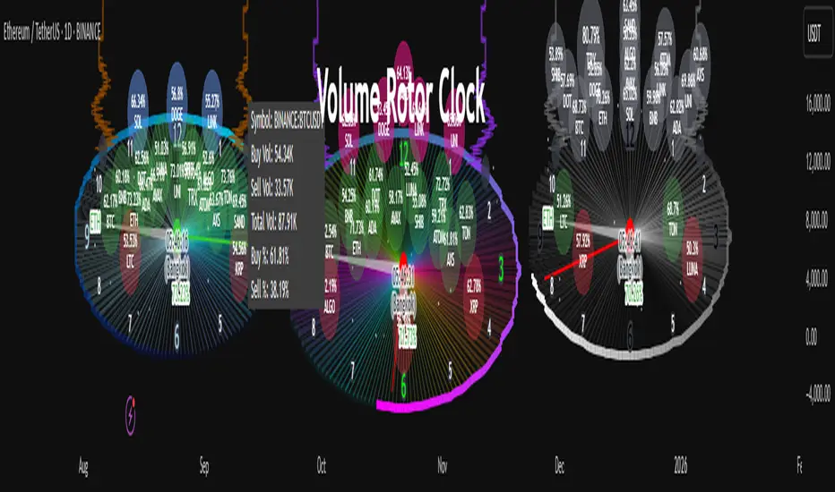
Prime NumbersPrime Numbers highlights prime numbers (no surprise there 😅), tokens and the recent "active" feature in "input".
🔸 CONCEPTS
🔹 What are Prime Numbers?
A prime number (or a prime) is a natural number greater than 1 that is not a product of two smaller natural numbers.
Wikipedia: Prime number
🔹 Prime Factorization
The fundamental theorem of arithmetic states that every integer larger than 1 can be written as a product of one or more primes. More strongly, this product is unique in the sense that any two prime factorizations of the same number will have the same number of copies of the same primes, although their ordering may differ. So, although there are many different ways of finding a factorization using an integer factorization algorithm, they all must produce the same result. Primes can thus be considered the "basic building blocks" of the natural numbers.
Wikipedia: Fundamental theorem of arithmetic
Math Is Fun: Prime Factorization
We divide a given number by Prime Numbers until only Primes remain.
Example:
24 / 2 = 12 | 24 / 3 = 8
12 / 3 = 4 | 8 / 2 = 4
4 / 2 = 2 | 4 / 2 = 2
|
24 = 2 x 3 x 2 | 24 = 3 x 2 x 2
or | or
24 = 2² x 3 | 24 = 2² x 3
In other words, every natural/integer number above 1 has a unique representation as a product of prime numbers, no matter how the number is divided. Only the order can change, but the factors (the basic elements) are always the same.
🔸 USAGE
The Prime Numbers publication contains two use cases:
Prime Factorization: performed on "close" prices, or a manual chosen number.
List Prime Numbers: shows a list of Prime Numbers.
The other two options are discussed in the DETAILS chapter:
Prime Factorization Without Arrays
Find Prime Numbers
🔹 Prime Factorization
Users can choose to perform Prime Factorization on close prices or a manually given number.
❗️ Note that this option only applies to close prices above 1, which are also rounded since Prime Factorization can only be performed on natural (integer) numbers above 1.
In the image below, the left example shows Prime Factorization performed on each close price for the latest 50 bars (which is set with "Run script only on 'Last x Bars'" -> 50).
The right example shows Prime Factorization performed on a manually given number, in this case "1,340,011". This is done only on the last bar.
When the "Source" option "close price" is chosen, one can toggle "Also current price", where both the historical and the latest current price are factored. If disabled, only historical prices are factored.
Note that, depending on the chosen options, only applicable settings are available, due to a recent feature, namely the parameter "active" in settings.
Setting the "Source" option to "Manual - Limited" will factorize any given number between 1 and 1,340,011, the latter being the highest value in the available arrays with primes.
Setting to "Manual - Not Limited" enables the user to enter a higher number. If all factors of the manual entered number are in the 1 - 1,340,011 range, these factors will be shown; however, if a factor is higher than 1,340,011, the calculation will stop, after which a warning is shown:
The calculated factors are displayed as a label where identical factors are simplified with an exponent notation in superscript.
For example 2 x 2 x 2 x 5 x 7 x 7 will be noted as 2³ x 5 x 7²
🔹 List Prime Numbers
The "List Prime Numbers" option enables users to enter a number, where the first found Prime Number is shown, together with the next x Prime Numbers ("Amount", max. 200)
The highest shown Prime Number is 1,340,011.
One can set the number of shown columns to customize the displayed numbers ("Max. columns", max. 20).
🔸 DETAILS
The Prime Numbers publication consists out of 4 parts:
Prime Factorization Without Arrays
Prime Factorization
List Prime Numbers
Find Prime Numbers
The usage of "Prime Factorization" and "List Prime Numbers" is explained above.
🔹 Prime Factorization Without Arrays
This option is only there to highlight a hurdle while performing Prime Factorization.
The basic method of Prime Factorization is to divide the base number by 2, 3, ... until the result is an integer number. Continue until the remaining number and its factors are all primes.
The division should be done by primes, but then you need to know which one is a prime.
In practice, one performs a loop from 2 to the base number.
Example:
Base_number = input.int(24)
arr = array.new()
n = Base_number
go = true
while go
for i = 2 to n
if n % i == 0
if n / i == 1
go := false
arr.push(i)
label.new(bar_index, high, str.tostring(arr))
else
arr.push(i)
n /= i
break
Small numbers won't cause issues, but when performing the calculations on, for example, 124,001 and a timeframe of, for example, 1 hour, the script will struggle and finally give a runtime error.
How to solve this?
If we use an array with only primes, we need fewer calculations since if we divide by a non-prime number, we have to divide further until all factors are primes.
I've filled arrays with prime numbers and made libraries of them. (see chapter "Find Prime Numbers" to know how these primes were found).
🔹 Tokens
A hurdle was to fill the libraries with as many prime numbers as possible.
Initially, the maximum token limit of a library was 80K.
Very recently, that limit was lifted to 100K. Kudos to the TradingView developers!
What are tokens?
Tokens are the smallest elements of a program that are meaningful to the compiler. They are also known as the fundamental building blocks of the program.
I have included a code block below the publication code (// - - - Educational (2) - - - ) which, if copied and made to a library, will contain exactly 100K tokens.
Adding more exported functions will throw a "too many tokens" error when saving the library. Subtracting 100K from the shown amount of tokens gives you the amount of used tokens for that particular function.
In that way, one can experiment with the impact of each code addition in terms of tokens.
For example adding the following code in the library:
export a() => a = array.from(1) will result in a 100,041 tokens error, in other words (100,041 - 100,000) that functions contains 41 tokens.
Some more examples, some are straightforward, others are not )
// adding these lines in one of the arrays results in x tokens
, 1 // 2 tokens
, 111, 111, 111 // 12 tokens
, 1111 // 5 tokens
, 111111111 // 10 tokens
, 1111111111111111111 // 20 tokens
, 1234567890123456789 // 20 tokens
, 1111111111111111111 + 1 // 20 tokens
, 1111111111111111111 + 8 // 20 tokens
, 1111111111111111111 + 9 // 20 tokens
, 1111111111111111111 * 1 // 20 tokens
, 1111111111111111111 * 9 // 21 tokens
, 9999999999999999999 // 21 tokens
, 1111111111111111111 * 10 // 21 tokens
, 11111111111111111110 // 21 tokens
//adding these functions to the library results in x tokens
export f() => 1 // 4 tokens
export f() => v = 1 // 4 tokens
export f() => var v = 1 // 4 tokens
export f() => var v = 1, v // 4 tokens
//adding these functions to the library results in x tokens
export a() => const arraya = array.from(1) // 42 tokens
export a() => arraya = array.from(1) // 42 tokens
export a() => a = array.from(1) // 41 tokens
export a() => array.from(1) // 32 tokens
export a() => a = array.new() // 44 tokens
export a() => a = array.new(), a.push(1) // 56 tokens
What if we could lower the amount of tokens, so we can export more Prime Numbers?
Look at this example:
829111, 829121, 829123, 829151, 829159, 829177, 829187, 829193
Eight numbers contain the same number 8291.
If we make a function that removes recurrent values, we get fewer tokens!
829111, 829121, 829123, 829151, 829159, 829177, 829187, 829193
//is transformed to:
829111, 21, 23, 51, 59, 77, 87, 93
The code block below the publication code (// - - - Educational (1) - - - ) shows how these values were reduced. With each step of 100, only the first Prime Number is shown fully.
This function could be enhanced even more to reduce recurrent thousands, tens of thousands, etc.
Using this technique enables us to export more Prime Numbers. The number of necessary libraries was reduced to half or less.
The reduced Prime Numbers are restored using the restoreValues() function, found in the library fikira/Primes_4.
🔹 Find Prime Numbers
This function is merely added to show how I filled arrays with Prime Numbers, which were, in turn, added to libraries (after reduction of recurrent values).
To know whether a number is a Prime Number, we divide the given number by values of the Primes array (Primes 2 -> max. 1,340,011). Once the division results in an integer, where the divisor is smaller than the dividend, the calculation stops since the given number is not a Prime.
When we perform these calculations in a loop, we can check whether a series of numbers is a Prime or not. Each time a number is proven not to be a Prime, the loop starts again with a higher number. Once all Primes of the array are used without the result being an integer, we have found a new Prime Number, which is added to the array.
Doing such calculations on one bar will result in a runtime error.
To solve this, the findPrimeNumbers() function remembers the index of the array. Once a limit has been reached on 1 bar (for example, the number of iterations), calculations will stop on that bar and restart on the next bar.
This spreads the workload over several bars, making it possible to continue these calculations without a runtime error.
The result is placed in log.info() , which can be copied and pasted into a hardcoded array of Prime Number values.
These settings adjust the amount of workload per bar:
Max Size: maximum size of Primes array.
Max Bars Runtime: maximum amount of bars where the function is called.
Max Numbers To Process Per Bar: maximum numbers to check on each bar, whether they are Prime Numbers.
Max Iterations Per Bar: maximum loop calculations per bar.
🔹 The End
❗️ The code and description is written without the help of an LLM, I've only used Grammarly to improve my description (without AI :) )
