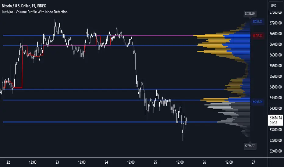
Volume Profile with Node Detection [LuxAlgo]The Volume Profile with Node Detection is a charting tool that allows visualizing the distribution of traded volume across specific price levels and highlights significant volume nodes or clusters of volume nodes that traders may find relevant in utilizing in their trading strategies.
🔶 USAGE
The volume profile component of the script serves as the foundation for node detection while encompassing all the essential features expected from a volume profile. See the sub-sections below for more detailed information about the indicator components and their usage.
🔹 Peak Volume Node Detection
A volume peak node is identified when the volume profile nodes for the N preceding and N succeeding nodes are lower than that of the evaluated one.
Displaying peak volume nodes along with their surrounding N nodes (Zones or Clusters) helps visualize the range, typically representing consolidation zones in the market. This feature enables traders to identify areas where trading activity has intensified, potentially signaling periods of price consolidation or indecision among market participants.
🔹 Trough Volume Node Detection
A volume trough node is identified when the volume profile nodes for the N preceding and N succeeding nodes are higher than that of the evaluated one.
🔹 Highest and Lowest Volume Nodes
Both the highest and lowest volume areas play significant roles in trading. The highest volume areas typically represent zones of strong price acceptance, where a significant amount of trading activity has occurred. On the other hand, the lowest volume areas signify price levels with minimal trading activity, often indicating zones of price rejection or areas where market participants have shown less interest.
🔹 Volume profile
Volume profile is calculated based on the volume of trades that occur at various price levels within a specified timeframe. It divides the price range into discrete price intervals, typically known as "price buckets" or "price bars," and then calculates the total volume of trades that occur at each price level within those intervals. This information is then presented graphically as a histogram or profile, where the height of each bar represents the volume of trades that occurred at that particular price level.
🔶 SETTINGS
🔹 Volume Nodes
Volume Peaks: Toggles the visibility of either the "Peaks" or "Clusters" on the chart, depending on the specified percentage for detection.
Node Detection Percent %: Specifies the percentage for the Volume Peaks calculation.
Volume Troughs: Toggles the visibility of either the "Troughs" or "Clusters" on the chart, depending on the specified percentage for detection.
Node Detection Percent %: Specifies the percentage for the Volume Troughs calculation.
Volume Node Threshold %: A threshold value specified as a percentage is utilized to detect peak/trough volume nodes. If a value is set, the detection will disregard volume node values lower than the specified threshold.
Highest Volume Nodes: Toggles the visibility of the highest nodes for the specified count.
Lowest Volume Nodes: Toggles the visibility of the lowest nodes for the specified count.
🔹 Volume Profile - Components
Volume Profile: Toggles the visibility of the volume profile with either classical display or gradient display.
Value Area Up / Down: Color customization option for the volume nodes within the value area of the profile.
Profile Up / Down Volume: Color customization option for the volume nodes outside of the value area of the profile.
Point of Control: Toggles the visibility of the point of control, allowing selection between "developing" or "regular" modes. Sets the color and width of the point of control line accordingly.
Value Area High (VAH): Toggles the visibility of the value area high level and allows customization of the line color.
Value Area Low (VAL): Toggles the visibility of the value area low level and allows customization of the line color.
Profile Price Labels: Toggles the visibility of the Profile Price Levels and allows customization of the text size of the levels.
🔹 Volume Profile - Display Settings
Profile Lookback Length: Specifies the length of the profile lookback period.
Value Area (%): Specifies the percentage for calculating the value area.
Profile Placement: Specify where to display the profile.
Profile Number of Rows: Specify the number of rows the profile will have.
Profile Width %: Adjusts the width of the rows in the profile relative to the profile range.
Profile Horizontal Offset: Adjusts the horizontal offset of the profile when it is selected to be displayed on the right side of the chart.
Value Area Background: Toggles the visibility of the value area background and allows customization of the fill color.
Profile Background: Toggles the visibility of the profile background and allows customization of the fill color.
🔶 RELATED SCRIPTS
Supply-Demand-Profiles
Liquidity-Sentiment-Profile
Thanks to our community for recommending this script. For more conceptual scripts and related content, we welcome you to explore by visiting >>> LuxAlgo-Scripts .
스크립트에서 "THE SCRIPT"에 대해 찾기
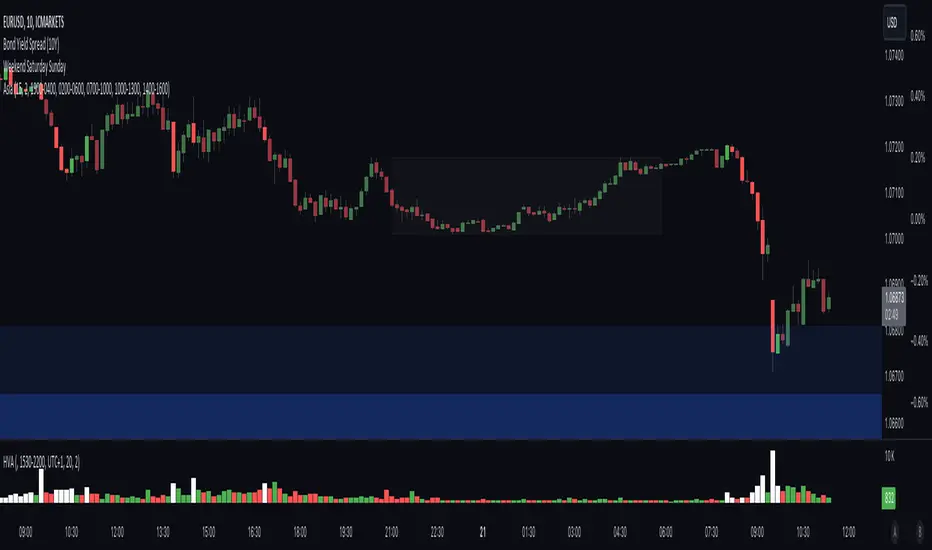
High Volume AlertThe High Volume Alert Script is developed for all traders focusing on volume analysis in their trading strategies, providing alerts for unusually high trading volumes during specified trading sessions.
Functionality:
Volume Moving Average Calculation:
Average Volume = Moving Average(Volume) = Sum of last the x last candles Volume
Where n is the user-defined period for the moving average calculation (denoted as movingaverageinput in the script. This moving average serves as the baseline to compare current volume levels against historical averages.
High Volume Detection:
HighVolume = CurrentVolume >= (MA(Volume) x HighVolumeRatio)
Here, HighVolumeRatio is a user-defined multiplier that sets the threshold for what is considered high volume. If the current volume exceeds this threshold (the product of the moving average of volume and the HighVolumeRatio ), the script identifies this as a high-volume event.
Session Filtering:
The script further refines these alerts by ensuring they only trigger during the specified trading session, enhancing relevance for traders interested in specific market hours. This session is defined by the sess and timezone parameters.
Visualisation and Alerts:
If high volume is detected (HighVolume = True), the script colors the volume bar with the highVolumeColor . If the option is selected, it also changes the color of the candlestick to either highVolumeCandleColorUp (for bullish candles) or highVolumeCandleColorDown (for bearish candles), depending on the price movement within the high-volume period. An alert is generated through the alertcondition function when high volume is detected during the specified session, notifying the trader of potentially significant market activity.
Application in Trading:
This indicator serves traders who prioritize volume as a leading indicator of potential price movement. High trading volumes may indicate the presence of significant market activity, often associated with events like news releases, market openings, or large trades, which can precede price movements.
Originality and Practicality:
This script is self-developed, aiming to fill the gap in automatic ratio adjusted volume alerts within the TradingView environment.
Conclusion:
The High Volume Alert Script is an essential tool for traders who integrate volume analysis into their strategy, offering tailored alerts and visual cues for high volume periods.
Compliance and Limitations:
The script complies with TradingView scripting standards, ensuring no lookahead bias and maintaining real-time data integrity. However, its utility depends on the availability on volume data, and please be aware that forex pairs never offer real volume data, this tool is best used with a exchange traded symbol.
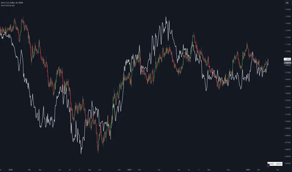
Bond Yield SpreadThe Bond Yield Spread Script is developed for forex traders, offering an automated tool to calculate the bond yield spread between two countries associated with the forex pair displayed on the chart.
Functionality:
The script starts by identifying the base and quote currencies of the current forex pair and aligns them with their corresponding national bond symbols based on user-selected maturity, with options ranging from 01Y to 30Y. It calculates the yield spread by subtracting the bond yield associated with the quote country from that of the base country, following the formula:
Yield Spread = Yield(Base Country) − Yield(Quote Country)
which is then displayed as a plot line on the chart.
This script relies solely on TradingView's internal yield symbols, with the following calculation:
"currency" => "first two letters" + maturity
And maturity, in this case, is the value that is configured in the indicator settings, for example:
"EUR" => "EU" + "02Y" will result in EU02Y -> which will be used in the formula, depending on the quote or base currency.
Application in Trading:
This indicator is invaluable for traders employing carry trading strategies or assessing currency strength based on traded interest rates as an indicator. A higher yield spread typically indicates a stronger currency, because the return obtained for holding the currency is higher.
Originality and Practicality:
This script is self-developed, aiming to fill the gap in automatic bond yield comparisons within the TradingView environment. It is particularly beneficial for traders focusing on macroeconomic factors affecting forex markets. Unlike other scripts, it integrates various bond maturities into one tool, enhancing its utility and application range.
Conclusion:
Designed for traders incorporating macroeconomics in their strategy, this script will be useful to calculate the bond yield differences automatically without having to enter a new formula for every new currency pair.
Compliance and Limitations:
The script complies with TradingView scripting standards, ensuring no lookahead bias and maintaining real-time data integrity. However, its utility depends on the comprehensive availability of bond yield data within TradingView. As not all countries issue bonds for each listed maturity, this may limit the script’s application for certain currency pairs or specific maturities.
RAINBOW AVERAGES - INDICATOR - (AS) - 1/3
-INTRODUCTION:
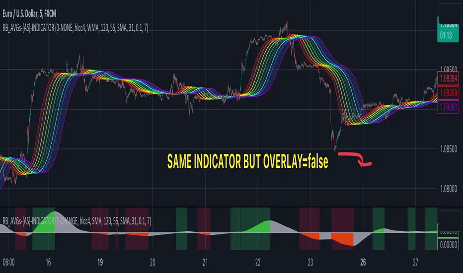
This is the first of three scripts I intend to publish using rainbow indicators. This script serves as a groundwork for the other two. It is a RAINBOW MOVING AVERAGES indicator primarily designed for trend detection. The upcoming script will also be an indicator but with overlay=false (below the chart, not on it) and will utilize RAINBOW BANDS and RAINBOW OSCILLATOR. The third script will be a strategy combining all of them.
RAINBOW moving averages can be used in various ways, but this script is mainly intended for trend analysis. It is meant to be used with overlay=true, but if the user wishes, it can be viewed below the chart. To achieve this, you need to change the code from overlay=true to false and turn off the first switch that plots the rainbow on the chart (or simply move the indicator to a new pane below). By doing this, you will be able to see how all four conditions used to detect trends work on the chart. But let's not get ahead of ourselves.
-WHAT IS IT:
In its simplest form, this indicator uses 10 moving averages colored like a rainbow. The calculation is as follows:
MA0: This is the main moving average and can be defined with the type (SMA, EMA, RMA, WMA, SINE), length, and price source. However, the second moving average (MA1) is calculated using MA0 as its source, MA2 uses MA1 as the data source, and so on, until the last one, MA9. Hence, there are 10 moving averages. The first moving average is special as all the others derive from it. This indicator has many potential uses, such as entry/exit signals, volatility indication, and stop-loss placement, but for now, we will focus on trend detection.
-TREND DETECTION:
The indicator offers four different background color options based on the user's preference:
0-NONE: No background color is applied as no trend detection tools is being used (boring)
1-CHANGE: The background color is determined by summing the changes of all 10 moving averages (from two bars). If the sum is positive and not falling, the background color is GREEN. If the sum is negative and not rising, the background color is RED. From early testing, it works well for the beginning of a movement but not so much for a lasting trend.
2-RAINBW: The background color is green when all the moving averages are in ascending order, indicating a bullish trend. It is red when all the moving averages are in descending order, indicating a bearish trend. For example, if MA1>MA2>MA3>MA4..., the background color is green. If MA1 threshold, and red indicates width < -threshold.
4-DIRECT: The background color is determined by counting the number of moving averages that are either above or below the input source. If the specified number of moving averages is above the source, the background color is green. If the specified number of moving averages is below the source, the background color is red. If all ten MAs are below the price source, the indicator will show 10, and if all ten MAs are above, it will show -10. The specific value will be set later in the settings (same for 3-TSHOLD variant). This method works well for lasting trends.
Note: If the indicator is turned into a below-chart version, all four color options can be seen as separate indicators.
-PARAMETERS - SETTINGS:
The first line is an on/off switch to plot the skittles indicator (and some info in the tooltip). The second line has already been discussed, which is the background color and the selection of the source (only used for MA0!).
The line "MA1: TYP/LEN" is where we define the parameters of MA0 (important). We choose from the types of moving averages (SMA, EMA, RMA, WMA, SINE) and set the length.
Important Note: It says MA1, but it should be MA0!.
The next line defines whether we want to smooth MA1 (which is actually MA0) and the period for smoothing. When smoothing is turned on, MA0 will be smoothed using a 3-pole super smoother. It's worth noting that although this only applies to MA0, as the other MAs are derived from it, they will also be smoothed.
In the line below, we define the type and length of MAs for MA2 (and other MAs except MA0). The same type and length are used for MA1 to MA9. It's important to remember that these values should be smaller. For example, if we set 55, it means that MA1 is the average of 55 periods of MA0, MA2 will be 55 periods of MA1, and so on. I encourage trying different combinations of MA types as it can be easily adjusted for ur type of trading. RMA looks quirky.
Moving on to the last line, we define some inputs for the background color:
TSH: The threshold value when using 3-TSHOLD-BGC. It's a good idea to change the chart to a pane below for easier adjustment. The default values are based on EURUSD-5M.
BG_DIR: The value that must be crossed or equal to the MA score if using 4-DIRECT-BGC. There are 10 MAs, so the maximum value is also 10. For example, if you set it to 9, it means that at least 9 MAs must be below/above the price for the script to detect a trend. Higher values are recommended as most of the time, this indicator oscillates either around the maximum or minimum value.
-SUMMARY OF SETTINGS:
L1 - PLOT MAs and general info tooltip
L2 - Select the source for MA0 and type of trend detection.
L3 - Set the type and length of MA0 (important).
L4 - Turn smoothing on/off for MA0 and set the period for super smoothing.
L5 - Set the type and length for the rest of the MAs.
L6 - Set values if using 4-DIRECT or 3-TSHOLD for the trend detection.
-OTHERS:
To see trend indicators, you need to turn off the plotting of MAs (first line), and then choose the variant you want for the background color. This will plot it on the chart below.
Keep in mind that M1 int settings stands for MA0 and MA2 for all of the 9 MAs left.
Yes, it may seem more complicated than it actually is. In a nutshell, these are 10 MAs, and each one after MA0 uses the previous one as its source. Plus few conditions for range detection. rest is mainly plots and colors.
There are tooltips to help you with the parameters.
I hope this will be useful to someone. If you have any ideas, feedback, or spot errors in the code, LET ME KNOW.
Stay tuned for the remaining two scripts using skittles indicators and check out my other scripts.
-ALSO:
I'm always looking for ideas for interesting indicators and strategies that I could code, so if you don't know Pinescript, just message me, and I would be glad to write your own indicator/strategy for free, obviously.
-----May the force of the market be with you, and until we meet again,
™TradeChartist Fib Extensions™TradeChartist Fib Extensions is a free to use script that helps traders plot Fibonacci Extensions on chart. Even though Trading View has a Fib extensions tool, some traders may prefer a plotting script like this with Fib plot lines extending across the whole of the chart to track historic prices in relation to Fib extensions drawn.
----To draw Fib extensions for uptrend ,
1. Choose a Pivot Low point (LL or a HL) as Pivot 1
2. Choose a Pivot High point (must be higher than Pivot 1) as Pivot 2
3. Choose a Pivot Low point (must be lower than Pivot 2, must be Higher than Pivot 1)
----To draw Fib extensions for downtrend,
1. Choose a Pivot High point (HH or a LH) as Pivot 1
2. Choose a Pivot Low point (must be lower than Pivot 1) as Pivot 2
3. Choose a Pivot High point (must be higher than Pivot 2 and lower than Pivot 1)
Negative extensions of -23.6% and -61.8% fib plots may be useful for some to spot reversals or to set stop losses.
Higher levels can be used if price goes beyond 161.8%
This is a free to use indicator. Give a thumbs up or leave a comment if you like the script
Check my 'Scripts' page to see other published scripts. Get in touch with me if you would like access to my invite-only scripts for a trial before deciding on a paid access for a period of your choice. Half-Yearly, Annual and Lifetime access available on invite-only scripts along with 1hr Team Viewer intro session.

Volume essential parameters overlayVolume EPO – Essential Volume Parameters Overlay
1. Motivation and design philosophy
Volume EPO is designed as a conceptual overlay rather than a self contained trading system. The main idea behind this script is to take complex, foundational market concepts out of heavy, menu driven strategies and express them as lightweight, independent layers that sit on top of any chart or indicator.
In many TradingView scripts, a single strategy tries to handle everything at once: signal logic, risk settings, visual cues, multi timeframe controls, and conceptual explanations. This usually leads to long input menus, performance issues, and difficult maintenance. The architectural approach behind Volume EPO is the opposite: keep the core strategy lean, and move the explanation and measurement of key concepts into dedicated overlays.
In this framework, Volume EPO is the base layer for the concept of volume. It does not decide anything about entries or exits. Instead, it exposes and clarifies how different definitions of volume behave candle by candle. Other layers or strategies can then build on top of this understanding.
2. What Volume EPO does
Volume EPO focuses on four essential volume parameters for each bar:
- Buy volume - Sell volume - Total volume - Delta volume (the difference between buy and sell volume)
The script presents these parameters in a compact heads up display (HUD) table that can be positioned anywhere on the chart. It is designed to be visually minimal, language aware, and usable on top of any other indicator or price action without cluttering the view.
The indicator does not output signals, alerts, arrows, or strategy entries. It is a descriptive and educational tool that shows how volume is distributed, not a prescriptive tool that tells the trader what to do.
3. Two definitions of volume
A central theme of this script is that there is more than one way to define and interpret “volume” inside a single candle. Volume EPO implements and clearly separates two different approaches:
- A geometric, candle based approximation that uses only OHLC and volume of the current bar. - An intrabar, data driven definition that uses lower timeframe up and down volume when it is available.
The user can switch between these modes via the calculation method input. The mode is prominently shown inside the on chart table so that the context is always explicit.
3.1 Geometry mode (Source File, approximate)
In Geometry mode, Volume EPO works only with the current bar’s OHLC values and total volume. No lower timeframe data is required.
The candle’s range is defined as high minus low. If the range is positive, the position of the close inside that range is used as a simple model for how volume might have been distributed between buyers and sellers:
- The closer the close is to the high, the more of the total volume is attributed to the buying side. - The closer the close is to the low, the more of the total volume is attributed to the selling side. - In a rare case where the bar has no price range (for example a flat or doji bar), total volume is split evenly between buy and sell volume.
From this model, the script derives:
- Buy volume (approximated) - Sell volume (approximated) - Total volume (as reported by the bar) - Delta volume as the difference between buy and sell volume
This approach is intentionally labeled as “Geometry (Approx)” in the HUD. It is a theoretical reconstruction based solely on the candle’s geometry and total volume, and it is always available on any market or timeframe that provides OHLCV data.
3.2 Intrabar mode (Precise)
In Intrabar mode, Volume EPO uses the TradingView built in library for up and down volume on a user selected lower timeframe. Instead of inferring volume from the shape of the candle, it reads the underlying lower timeframe data when that data is accessible.
The script requests up and down volume from a lower timeframe such as 15 seconds, using the official TA library functions. The results are then interpreted as follows:
- Buy volume is taken as the absolute value of the up volume. - Sell volume is taken as the absolute value of the down volume. - Total volume is the sum of buy and sell volume. - Delta volume is provided directly by the library as the difference between up and down volume.
If valid lower timeframe data exists for a bar, the bar is counted as covered by Intrabar data. If not, that bar is marked as invalid for this precise calculation and is excluded from the covered count.
This mode is labeled “Precise” in the HUD, together with the selected lower timeframe, because it is anchored in actual intrabar data rather than in a geometric model. It provides a closer view of how buying and selling pressure unfolded inside the bar, at the cost of requiring more data and being dependent on the availability of that data.
4. Coverage, lookback, and what the numbers mean
The top part of the HUD reports not only which volume definition is active, but also an additional line that describes the effective coverage of the data.
In Intrabar (Precise) mode, the script displays:
- “Scanned: N Bars”
Here, N counts how many bars since the indicator was loaded have successfully received valid lower timeframe delta data. It is a measure of how much of the visible history has been truly covered by intrabar information, not a lookback window in the sense of a rolling calculation.
In Geometry mode, the script displays:
- “Lookback: L Bars”
In this extracted layer, the lookback value L is purely descriptive. It does not change how the current bar’s volume is computed, and it is not used in any iterative or statistical calculation inside this script. It is meant as a conceptual label, for example to keep the volume layer consistent with a broader framework where lookback length is a structural parameter.
Summarizing these two fields:
- Scanned tells you how many bars have been processed using real intrabar data. - Lookback is a descriptive parameter in Geometry mode in this specific overlay, not a direct driver of the computations.
5. The HUD layout on the chart
The on chart table is intentionally compact and structured to be read quickly:
- Header: a title identifying the overlay as Volume EPO. - Mode line: explicitly states whether the script is in Precise or Geometry mode, and for Precise mode also shows the lower timeframe used. - Coverage line: - In Precise mode, it shows “Scanned: N Bars”. - In Geometry mode, it shows “Lookback: L Bars”. - Volume block: - A line for buy and sell volume, marked with clear directional symbols. - A line for total volume and the absolute delta, accompanied by the sign of the delta. - Numeric formatting uses human friendly suffixes (for example K, M, B) to keep the display readable. - Footer: the current symbol and a time stamp, adjusted by a user selectable timezone offset so that the HUD can be aligned with the trader’s local time reference.
The table can be positioned anywhere on the chart and resized via inputs, and it supports multiple color themes and languages in order to integrate cleanly into different chart layouts.
6. How to use Volume EPO in practice
Volume EPO is meant to be read together with price action and other tools, not in isolation. Typical uses include:
- Studying how often a strong directional candle is actually supported by dominant buy or sell volume. - Comparing the behavior of delta volume between Geometry and Intrabar definitions. - Building a personal intuition for how intrabar data refines or contradicts the simple candle based approximation. - Feeding these insights into separate, lean strategy scripts that do not need to carry the full explanatory logic of volume inside them.
Because it is an overlay layer, Volume EPO can be stacked with other custom indicators without adding new signals or complexity to their logic. It simply adds a clear and consistent view of volume behavior on top of whatever the trader is already watching.
7. Educational and non signalling nature
Finally, it is important to stress that Volume EPO is not a trading system, not a signal generator, and not financial advice. The script does not tell the user when to enter or exit. It only reports how different definitions of volume describe the current bar.
Deciding whether to trade, how to trade, and which risk parameters to use remains entirely with the user and with their own strategy. Volume EPO provides context and clarity around the concept of volume so that those decisions can be informed by a better understanding of how buying and selling pressure is structured inside each candle.
Note: Even on lower timeframes, every reconstruction of volume remains an approximation, except at the true single tick level. However, the closer the chosen lower timeframe is to a one tick stream, the more accurately it can reflect the underlying order flow and balance between buying and selling pressure.

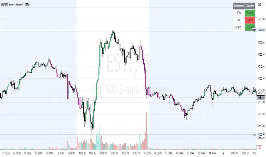
Multi-Timeframe Continuity Custom Candle ConfirmationMulti-Timeframe Continuity Custom Candle Confirmation
Overview
The Timeframe Continuity Indicator is a versatile tool designed to help traders identify alignment between their current chart’s candlestick direction and higher timeframes of their choice. By coloring bars on the current chart (e.g., 1-minute) based on the directional alignment with selected higher timeframes (e.g., 10-minute, daily), this indicator provides a visual cue for confirming trends across multiple timeframes—a concept known as Timeframe Continuity. This approach is particularly useful for day traders, swing traders, and scalpers looking to ensure their trades align with broader market trends, reducing the risk of trading against the prevailing momentum.
Originality and Usefulness
This indicator is an original creation, built from scratch to address a common challenge in trading: ensuring that price action on a lower timeframe aligns with the trend on higher timeframes. Unlike many trend-following indicators that rely on moving averages, oscillators, or other lagging metrics, this script directly compares the bullish or bearish direction of candlesticks across timeframes. It introduces the following unique features:
Customizable Timeframes: Users can select from a range of higher timeframes (5m, 10m, 15m, 30m, 1h, 2h, 4h, 1d, 1w, 1M) to check for alignment, making it adaptable to various trading styles.
Neutral Candle Handling: The script accounts for neutral candles (where close == open) on the current timeframe by allowing them to inherit the direction of the higher timeframe, ensuring continuity in trend visualization.
Table: A table displays the direction of each selected timeframe and the current timeframe, helping identify direction in the event you don't want to color bars.
Toggles for Flexibility: Options to disable bar coloring and the debug table allow users to customize the indicator’s visual output for cleaner charts or focused analysis.
This indicator is not a mashup of existing scripts but a purpose-built tool to visualize timeframe alignment directly through candlestick direction, offering traders a straightforward way to confirm trend consistency.
What It Does
The Timeframe Continuity Indicator colors bars on your chart when the direction of the current timeframe’s candlestick (bullish, bearish, or neutral) aligns with the direction of the selected higher timeframes:
Lime: The current bar (e.g., 1m) is bullish or neutral, and all selected higher timeframes (e.g., 10m) are bullish.
Pink: The current bar is bearish or neutral, and all selected higher timeframes are bearish.
Default Color: If the directions don’t align (e.g., 1m bar is bearish but 10m is bullish), the bar remains the default chart color.
The indicator also includes a debug table (toggleable) that shows the direction of each selected timeframe and the current timeframe, helping traders diagnose alignment issues.
How It Works
The script uses the following methodology:
1. Direction Calculation: For each timeframe (current and selected higher timeframes), the script determines the candlestick’s direction:
Bullish (1): close > open / Bearish (-1): close < open / Neutral (0): close == open
Higher timeframe directions are fetched using Pine Script’s request.security function, ensuring accurate data retrieval.
2. Alignment Check: The script checks if all selected higher timeframes are uniformly bullish (full_bullish) or bearish (full_bearish).
o A higher timeframe must have a clear direction (bullish or bearish) to trigger coloring. If any selected timeframe is neutral, alignment fails, and no coloring occurs.
3. Coloring Logic: The current bar is colored only if its direction aligns with the higher timeframes:
Lime if the higher timeframes are bullish and the current bar is bullish or neutral.
Maroon if the higher timeframes are bearish and the current bar is bearish or neutral.
If the current bar’s direction opposes the higher timeframe (e.g., 1m bearish, 10m bullish), the bar remains uncolored.
Users can disable bar coloring entirely via the settings, leaving bars in their default chart color.
4. Direction Table:
A table in the top-right corner (toggleable) displays the direction of each selected timeframe and the current timeframe, using color-coded labels (green for bullish, red for bearish, gray for neutral).
This feature helps traders understand why a bar is or isn’t colored, making the indicator accessible to users unfamiliar with Pine Script.
How to Use
1. Add the Indicator: Add the "Timeframe Continuity Indicator" to your chart in TradingView (e.g., a 1m chart of SPY).
2. Configure Settings:
Timeframe Selection: Check the boxes for the higher timeframes you want to compare against (default: 10m). Options include 5m, 10m, 15m, 30m, 1h, 2h, 4h, 1D, 1W, and 1M. Select multiple timeframes if you want to ensure alignment across all of them (e.g., 10m and 1d).
Enable Bar Coloring: Default: true (bars are colored lime or maroon when aligned). Set to false to disable coloring and keep the default chart colors.
Show Table: Default: true (table is displayed in the top-right corner). Set to false to hide the table for a cleaner chart.
3. Interpret the Output:
Colored Bars: Lime bars indicate the current bar (e.g., 1m) is bullish or neutral, and all selected higher timeframes are bullish. Maroon bars indicate the current bar is bearish or neutral, and all selected higher timeframes are bearish. Uncolored bars (default chart color) indicate a mismatch (e.g., 1m bar is bearish while 10m is bullish) or no coloring if disabled.
Direction Table: Check the table to see the direction of each selected timeframe and the current timeframe.
4. Example Use Case:
On a 1m chart of SPY, select the 10m timeframe.
If the 10m timeframe is bearish, 1m bars that are bearish or neutral will color maroon, confirming you’re trading with the higher timeframe’s trend.
If a 1m bar is bullish while the 10m is bearish, it remains uncolored, signaling a potential misalignment to avoid trading.
Underlying Concepts
The indicator is based on the concept of Timeframe Continuity, a strategy used by traders to ensure that price action on a lower timeframe aligns with the trend on higher timeframes. This reduces the risk of entering trades against the broader market direction. The script directly compares candlestick directions (bullish, bearish, or neutral) rather than relying on lagging indicators like moving averages or RSI, providing a real-time, price-action-based confirmation of trend alignment. The handling of neutral candles ensures that minor indecision on the lower timeframe doesn’t interrupt the visualization of the higher timeframe’s trend.
Why This Indicator?
Simplicity: Directly compares candlestick directions, avoiding complex calculations or lagging indicators.
Flexibility: Customizable timeframes and toggles cater to various trading strategies.
Transparency: The debug table makes the indicator’s logic accessible to all users, not just those who can read Pine Script.
Practicality: Helps traders confirm trend alignment, a key factor in successful trading across timeframes.
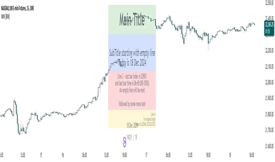
Watermark with dynamic variables [BM]█ OVERVIEW
This indicator allows users to add highly customizable watermark messages to their charts. Perfect for branding, annotation, or displaying dynamic chart information, this script offers advanced customization options including dynamic variables, text formatting, and flexible positioning.
█ CONCEPTS
Watermarks are overlay messages on charts. This script introduces placeholders — special keywords wrapped in % signs — that dynamically replace themselves with chart-related data. These watermarks can enhance charts with context, timestamps, or branding.
█ FEATURES
Dynamic Variables : Replace placeholders with real-time data such as bar index, timestamps, and more.
Advanced Customization : Modify text size, color, background, and alignment.
Multiple Messages : Add up to four independent messages per group, with two groups supported (A and B).
Positioning Options : Place watermarks anywhere on the chart using predefined locations.
Timezone Support : Display timestamps in a preferred timezone with customizable formats.
█ INPUTS
The script offers comprehensive input options for customization. Each Watermark (A and B) contains identical inputs for configuration.
Watermark settings are divided into two levels:
Watermark-Level Settings
These settings apply to the entire watermark group (A/B):
Show Watermark: Toggle the visibility of the watermark group on the chart.
Position: Choose where the watermark group is displayed on the chart.
Reverse Line Order: Enable to reverse the order of the lines displayed in Watermark A.
Message-Level Settings
Each watermark contains up to four configurable messages. These messages can be independently customized with the following options:
Message Content: Enter the custom text to be displayed. You can include placeholders for dynamic data.
Text Size: Select from predefined sizes (Tiny, Small, Normal, Large, Huge) or specify a custom size.
Text Alignment and Colors:
- Adjust the alignment of the text (Left, Center, Right).
- Set text and background colors for better visibility.
Format Time: Enable time formatting for this watermark message and configure the format and timezone. The settings for each message include message content, text size, alignment, and more. Please refer to Formatting dates and times for more details on valid formatting tokens.
█ PLACEHOLDERS
Placeholders are special keywords surrounded by % signs, which the script dynamically replaces with specific chart-related data. These placeholders allow users to insert dynamic content, such as bar information or timestamps, into watermark messages.
Below is the complete list of currently available placeholders:
bar_index , barstate.isconfirmed , barstate.isfirst , barstate.ishistory , barstate.islast , barstate.islastconfirmedhistory , barstate.isnew , barstate.isrealtime , chart.is_heikinashi , chart.is_kagi , chart.is_linebreak , chart.is_pnf , chart.is_range , chart.is_renko , chart.is_standard , chart.left_visible_bar_time , chart.right_visible_bar_time , close , dayofmonth , dayofweek , dividends.future_amount , dividends.future_ex_date , dividends.future_pay_date , earnings.future_eps , earnings.future_period_end_time , earnings.future_revenue , earnings.future_time , high , hl2 , hlc3 , hlcc4 , hour , last_bar_index , last_bar_time , low , minute , month , ohlc4 , open , second , session.isfirstbar , session.isfirstbar_regular , session.islastbar , session.islastbar_regular , session.ismarket , session.ispostmarket , session.ispremarket , syminfo.basecurrency , syminfo.country , syminfo.currency , syminfo.description , syminfo.employees , syminfo.expiration_date , syminfo.industry , syminfo.main_tickerid , syminfo.mincontract , syminfo.minmove , syminfo.mintick , syminfo.pointvalue , syminfo.prefix , syminfo.pricescale , syminfo.recommendations_buy , syminfo.recommendations_buy_strong , syminfo.recommendations_date , syminfo.recommendations_hold , syminfo.recommendations_sell , syminfo.recommendations_sell_strong , syminfo.recommendations_total , syminfo.root , syminfo.sector , syminfo.session , syminfo.shareholders , syminfo.shares_outstanding_float , syminfo.shares_outstanding_total , syminfo.target_price_average , syminfo.target_price_date , syminfo.target_price_estimates , syminfo.target_price_high , syminfo.target_price_low , syminfo.target_price_median , syminfo.ticker , syminfo.tickerid , syminfo.timezone , syminfo.type , syminfo.volumetype , ta.accdist , ta.iii , ta.nvi , ta.obv , ta.pvi , ta.pvt , ta.tr , ta.vwap , ta.wad , ta.wvad , time , time_close , time_tradingday , timeframe.isdaily , timeframe.isdwm , timeframe.isintraday , timeframe.isminutes , timeframe.ismonthly , timeframe.isseconds , timeframe.isticks , timeframe.isweekly , timeframe.main_period , timeframe.multiplier , timeframe.period , timenow , volume , weekofyear , year
█ HOW TO USE
1 — Add the Script:
Apply "Watermark with dynamic variables " to your chart from the TradingView platform.
2 — Configure Inputs:
Open the script settings by clicking the gear icon next to the script's name.
Customize visibility, message content, and appearance for Watermark A and Watermark B.
3 — Utilize Placeholders:
Add placeholders like %bar_index% or %timenow% in the "Watermark - Message" fields to display dynamic data.
Empty lines in the message box are reflected on the chart, allowing you to shift text up or down.
Using \n in the message box translates to a new line on the chart.
4 — Preview Changes:
Adjust settings and view updates in real-time on your chart.
█ EXAMPLES
Branding
DodgyDD's charts
Debugging
█ LIMITATIONS
Only supports variables defined within the script.
Limited to four messages per watermark.
Visual alignment may vary across different chart resolutions or zoom levels.
Placeholder parsing relies on correct input formatting.
█ NOTES
This script is designed for users seeking enhanced chart annotation capabilities. It provides tools for dynamic, customizable watermarks but is not a replacement for chart objects like text labels or drawings. Please ensure placeholders are properly formatted for correct parsing.
Additionally, this script can be a valuable tool for Pine Script developers during debugging . By utilizing dynamic placeholders, developers can display real-time values of variables and chart data directly on their charts, enabling easier troubleshooting and code validation.
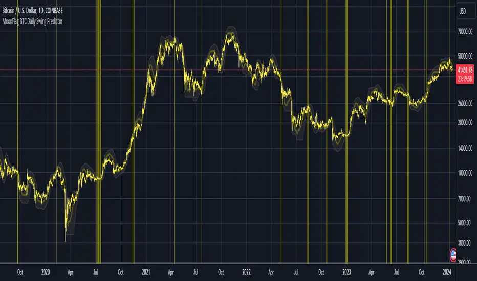
MoonFlag BTC Daily Swing PredictorThis script mainly works on BTC on the daily timeframe. Other coins also show similar usefulness with this script however, BTC on the daily timeframe is the main design for this script.
(Please note this is not trading advice this is just comments about how this indicator works.)
This script is predictive. It colors the background yellow when the script calculates a large BTC swing is potentially about to happen. It does not predict in which direction the swing will occur but it leads the price action so can be useful for leveraged trades. When the background gets colored with vertical yellow lines - this shows that a largish price swing is probably going to occur.
The scripts also shades bands around the price action that are used to estimate an acceptable volatility at any given time. If the bands are wide that means price action is volatile and large swings are not easily predicted. Over time, with reducing volatility, these price action bands narrow and then at a set point or percentage (%) which can be set in the script settings, the background gets colored yellow. This indicates present price action is not volatile and a large price swing is potentially going to happen in the near future. When price action breaks through the narrowing bands, the background is no longer presented because this is seen as an increase in volatility and a considerable portion of the time, a large sudden drop in price action or momentous gain in price is realized.
This indicator leads price action. It predicts that a swing is possibly going to happen in the near future. As the indicator works on the BTC daily, this means on a day-to-day basis if the bands continually narrow - a breakout is more likely to happen. In order to see how well this indicator works, have a look at the results on the screenshot provided. Note the regions where vertical yellow lines are present on the price action - and then look after these to see if a sizeable swing in price has occurred.
To use this indicator - wait until yellow vertical lines are presented on the BTC daily. Then use your experience to determine which way the price action might swing and consider entering a trade or leveraged trade in this direction. Alternatively wait a while to see in which direction the break-out occurs and considering and attempt to trade with this. Sometimes swings can be unexpected and breakout in one direction before then swinging much larger in the other. Its important to remember/consider that this indicator works on the BTC daily timeframe, so any consideration of entering a trade should be expected to cover a duration over many days or weeks, or possibly months. A large swing is only estimated every several plus months.
Most indicators are based on moving averages. A moving average is not predictive in the sense in that it lags price actions. This indicator creates bands that are based on the momentum of the price action. A change in momentum of price action therefore causes the bands to widen. When the bands narrow this means that the momentum of the price action is steady and price action volatility has converged/reduced over time. With BTC this generally means that a large swing in price action is going to occur as momentum in price action then pick-up again in one direction or another. Trying to view this using moving averages is not easy as a moving average lags price action which means that it is difficult to predict any sudden movements in price action ahead of when they might occur. Although, moving averages will converge over time in a similar manner as the bands calculated by this script. This script however, uses the price action momentum in a predictive manner to estimate where the price action might go based on present price momentum. This script therefore reacts to reduced volatility in price action much faster than a set of moving averages over various timescales can achieve.
MoonFlag
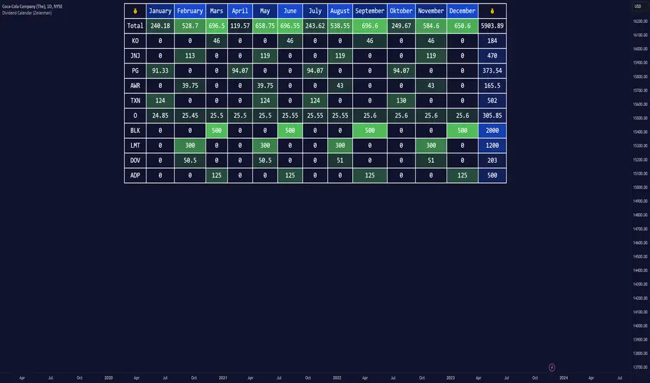
Dividend Calendar (Zeiierman)█ Overview
The Dividend Calendar is a financial tool designed for investors and analysts in the stock market. Its primary function is to provide a schedule of expected dividend payouts from various companies.
Dividends, which are portions of a company's earnings distributed to shareholders, represent a return on their investment. This calendar is particularly crucial for investors who prioritize dividend income, as it enables them to plan and manage their investment strategies with greater effectiveness. By offering a comprehensive overview of when dividends are due, the Dividend Calendar aids in informed decision-making, allowing investors to time their purchases and sales of stocks to optimize their dividend income. Additionally, it can be a valuable tool for forecasting cash flow and assessing the financial health and dividend-paying consistency of different companies.
█ How to Use
Dividend Yield Analysis:
By tracking dividend growth and payouts, traders can identify stocks with attractive dividend yields. This is particularly useful for income-focused investors who prioritize steady cash flow from their investments.
Income Planning:
For those relying on dividends as a source of income, the calendar helps in forecasting income.
Trend Identification:
Analyzing the growth rates of dividends helps in identifying long-term trends in a company's financial health. Consistently increasing dividends can be a sign of a company's strong financial position, while decreasing dividends might signal potential issues.
Portfolio Diversification:
The tool can assist in diversifying a portfolio by identifying a range of dividend-paying stocks across different sectors. This can help mitigate risk as different sectors may react differently to market conditions.
Timing Investments:
For those who follow a dividend capture strategy, this indicator can be invaluable. It can help in timing the buying and selling of stocks around their ex-dividend dates to maximize dividend income.
█ How it Works
This script is a comprehensive tool for tracking and analyzing stock dividend data. It calculates growth rates, monthly and yearly totals, and allows for custom date handling. Structured to be visually informative, it provides tables and alerts for the easy monitoring of dividend-paying stocks.
Data Retrieval and Estimation: It fetches dividend payout times and amounts for a list of stocks. The script also estimates future values based on historical data.
Growth Analysis: It calculates the average growth rate of dividend payments for each stock, providing insights into dividend consistency and growth over time.
Summation and Aggregation: The script sums up dividends on a monthly and yearly basis, allowing for a clear view of total payouts.
Customization and Alerts: Users can input custom months for dividend tracking. The script also generates alerts for upcoming or current dividend payouts.
Visualization: It produces various tables and visual representations, including full calendar views and income tables, to display the dividend data in an easily understandable format.
█ Settings
Overview:
Currency:
Description: This setting allows the user to specify the currency in which dividend values are displayed. By default, it's set to USD, but users can change it to their local currency.
Impact: Changing this value alters the currency denomination for all dividend values displayed by the script.
Ex-Date or Pay-Date:
Description: Users can select whether to show the Ex-dividend day or the Actual Payout day.
Impact: This changes the reference date for dividend data, affecting the timing of when dividends are shown as due or paid.
Estimate Forward:
Description: Enables traders to predict future dividends based on historical data.
Impact: When enabled, the script estimates future dividend payments, providing a forward-looking view of potential income.
Dividend Table Design:
Description: Choose between viewing the full dividend calendar, just the cumulative monthly dividend, or a summary view.
Impact: This alters the format and extent of the dividend data displayed, catering to different levels of detail a user might require.
Show Dividend Growth:
Description: Users can enable dividend growth tracking over a specified number of years.
Impact: When enabled, the script displays the growth rate of dividends over the selected number of years, providing insight into dividend trends.
Customize Stocks & User Inputs:
This setting allows users to customize the stocks they track, the number of shares they hold, the dividend payout amount, and the payout months.
Impact: Users can tailor the script to their specific portfolio, making the dividend data more relevant and personalized to their investments.
-----------------
Disclaimer
The information contained in my Scripts/Indicators/Ideas/Algos/Systems does not constitute financial advice or a solicitation to buy or sell any securities of any type. I will not accept liability for any loss or damage, including without limitation any loss of profit, which may arise directly or indirectly from the use of or reliance on such information.
All investments involve risk, and the past performance of a security, industry, sector, market, financial product, trading strategy, backtest, or individual's trading does not guarantee future results or returns. Investors are fully responsible for any investment decisions they make. Such decisions should be based solely on an evaluation of their financial circumstances, investment objectives, risk tolerance, and liquidity needs.
My Scripts/Indicators/Ideas/Algos/Systems are only for educational purposes!
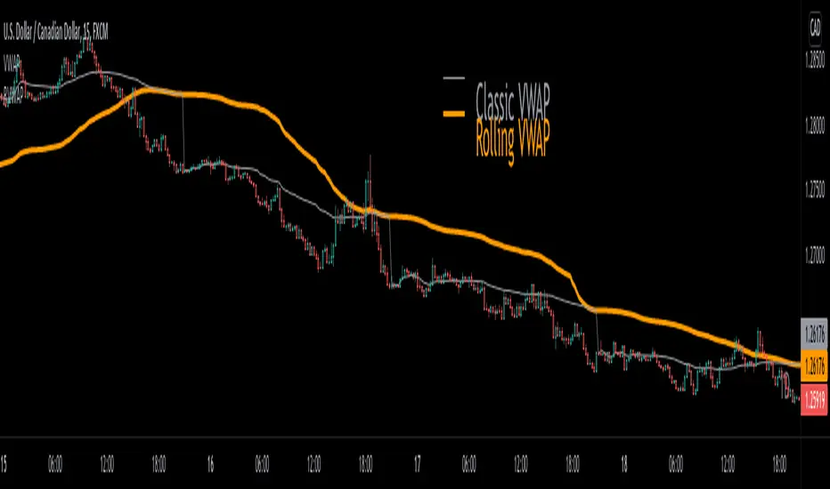
Rolling VWAP█ OVERVIEW
This indicator displays a Rolling Volume-Weighted Average Price. Contrary to VWAP indicators which reset at the beginning of a new time segment, RVWAP calculates using a moving window defined by a time period (not a simple number of bars), so it never resets.
█ CONCEPTS
If you are not already familiar with VWAP, our Help Center will get you started.
The typical VWAP is designed to be used on intraday charts, as it resets at the beginning of the day. Such VWAPs cannot be used on daily, weekly or monthly charts. Instead, this rolling VWAP uses a time period that automatically adjusts to the chart's timeframe. You can thus use RVWAP on any chart that includes volume information in its data feed.
Because RVWAP uses a moving window, it does not exhibit the jumpiness of VWAP plots that reset. You can see the more jagged VWAP on the chart above. We think both can be useful to traders; up to you to decide which flavor works for you.
█ HOW TO USE IT
Load the indicator on an active chart (see the Help Center if you don't know how).
Time period
By default, the script uses an auto-stepping mechanism to adjust the time period of its moving window to the chart's timeframe. The following table shows chart timeframes and the corresponding time period used by the script. When the chart's timeframe is less than or equal to the timeframe in the first column, the second column's time period is used to calculate RVWAP:
Chart Time
timeframe period
1min 🠆 1H
5min 🠆 4H
1H 🠆 1D
4H 🠆 3D
12H 🠆 1W
1D 🠆 1M
1W 🠆 3M
You can use the script's inputs to specify a fixed time period, which you can express in any combination of days, hours and minutes.
By default, the time period currently used is displayed in the lower-right corner of the chart. The script's inputs allow you to hide the display or change its size and location.
Minimum Window Size
This input field determines the minimum number of values to keep in the moving window, even if these values are outside the prescribed time period. This mitigates situations where a large time gap between two bars would cause the time window to be empty, which can occur in non-24x7 markets where large time gaps may separate contiguous chart bars, namely across holidays or trading sessions. For example, if you were using a 1D time period and there is a two-day gap between two bars, then no chart bars would fit in the moving window after the gap. The default value is 10 bars.
█ NOTES
If you are interested in VWAP indicators, you may find the VWAP Auto Anchored built-in indicator worth a try.
For Pine Script™ coders
The heart of this script's calculations uses the `totalForTimeWhen()` function from the ConditionalAverages library published by PineCoders . It works by maintaining an array of values included in a time period, but without a for loop requiring a lookback from the current bar, so it is much more efficient.
We write our Pine Script™ code using the recommendations in the User Manual's Style Guide .
Look first. Then leap.
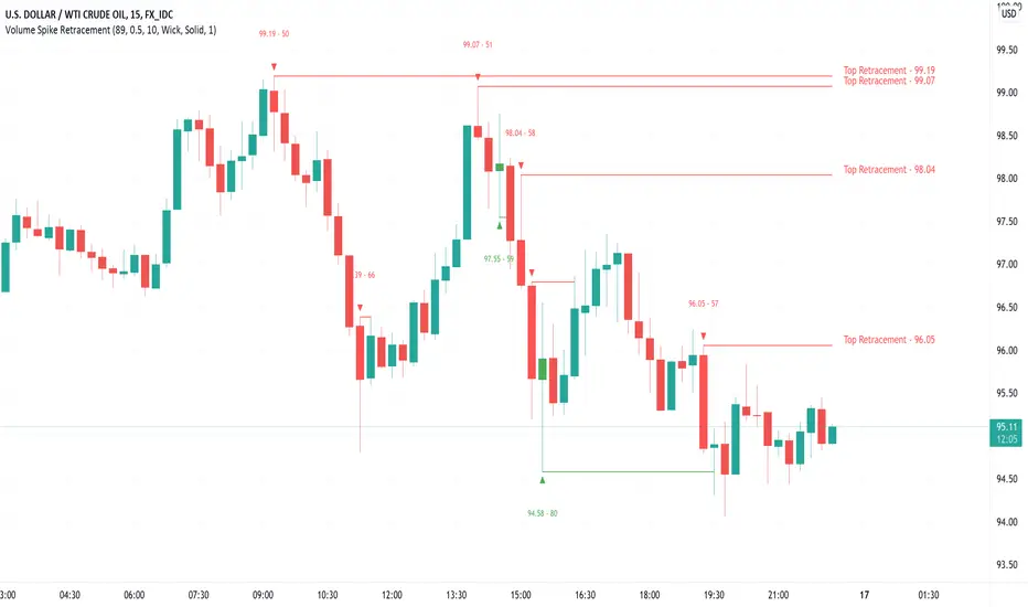
Volume Spike Retracement█ OVERVIEW
-Following many people's request to add "Volume" mode again in my "Institutional OrderBlock Pressure" script. I decided to release an improved
and full-fledged script. This will be the last OB/Retracement script I will release as we have explored every possible way to find them.
█ HOW TO INTERPRET?
-The script uses the the 0.5 Pivot and the maximum value set for Volume Length to find 'Peak Volume'. Once these conditions are met,
the script starts creating a Retracement Line.
-By default, the Volume Length value is set to 89, which works well with most Timeframes following the OrderBlocks/Retracements
logic used in my scripts.
-You have the option to set Alerts when the "Volume Spike Limit" is reached or when a Price Crossing with a Line occurs.
█ NOTES
- Yes Alerts appear instantly. Moreover, they are not 'confirmed', you must ALWAYS wait for confirmation before making a choice.
Good Trade everyone and remember, risk management remains the most important!
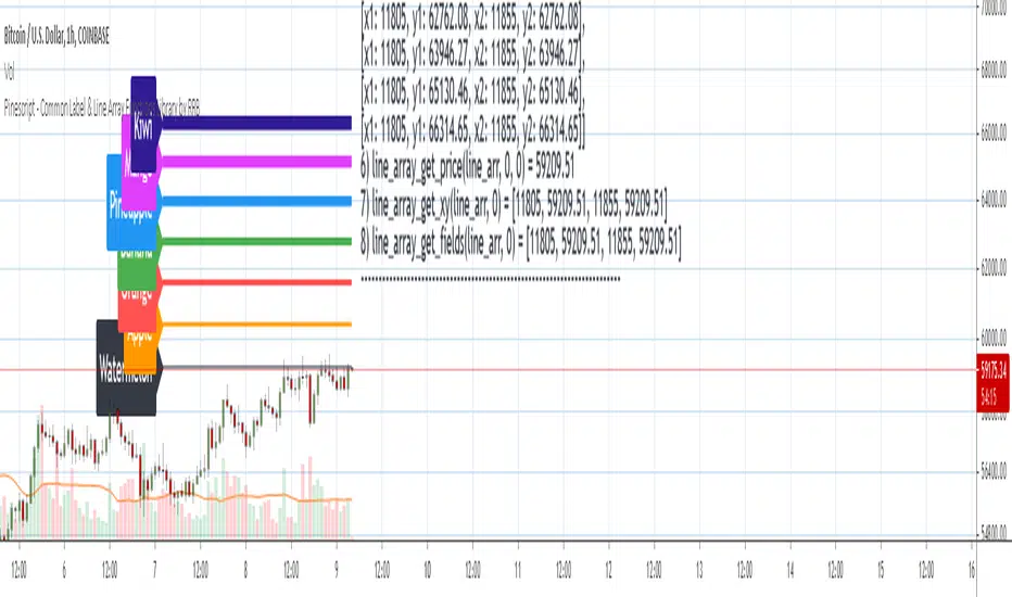
Pinescript - Common Label & Line Array Functions Library by RRBPinescript - Common Label & Line Array Functions Library by RagingRocketBull 2021
Version 1.0
This script provides a library of common array functions for arrays of label and line objects with live testing of all functions.
Using this library you can easily create, update, delete, join label/line object arrays, and get/set properties of individual label/line object array items.
You can find the full list of supported label/line array functions below.
There are several libraries:
- Common String Functions Library
- Standard Array Functions Library
- Common Fixed Type Array Functions Library
- Common Label & Line Array Functions Library
- Common Variable Type Array Functions Library
Features:
- 30 array functions in categories create/update/delete/join/get/set with support for both label/line objects (45+ including all implementations)
- Create, Update label/line object arrays from list/array params
- GET/SET properties of individual label/line array items by index
- Join label/line objects/arrays into a single string for output
- Supports User Input of x,y coords of 5 different types: abs/rel/rel%/inc/inc% list/array, auto transforms x,y input into list/array based on type, base and xloc, translates rel into abs bar indexes
- Supports User Input of lists with shortened names of string properties, auto expands all standard string properties to their full names for use in functions
- Live Output for all/selected functions based on User Input. Test any function for possible errors you may encounter before using in script.
- Output filters: hide all excluded and show only allowed functions using a list of function names
- Output Panel customization options: set custom style, color, text size, and line spacing
Usage:
- select create function - create label/line arrays from lists or arrays (optional). Doesn't affect the update functions. The only change in output should be function name regardless of the selected implementation.
- specify num_objects for both label/line arrays (default is 7)
- specify common anchor point settings x,y base/type for both label/line arrays and GET/SET items in Common Settings
- fill lists with items to use as inputs for create label/line array functions in Create Label/Line Arrays section
- specify label/line array item index and properties to SET in corresponding sections
- select label/line SET function to see the changes applied live
Code Structure:
- translate x,y depending on x,y type, base and xloc as specified in UI (required for all functions)
- expand all shortened standard property names to full names (required for create/update* from arrays and set* functions, not needed for create/update* from lists) to prevent errors in label.new and line.new
- create param arrays from string lists (required for create/update* from arrays and set* functions, not needed for create/update* from lists)
- create label/line array from string lists (property names are auto expanded) or param arrays (requires already expanded properties)
- update entire label/line array or
- get/set label/line array item properties by index
Transforming/Expanding Input values:
- for this script to work on any chart regardless of price/scale, all x*,y* are specified as % increase relative to x0,y0 base levels by default, but user can enter abs x,price values specific for that chart if necessary.
- all lists can be empty, contain 1 or several items, have the same/different lengths. Array Length = min(min(len(list*)), mum_objects) is used to create label/line objects. Missing list items are replaced with default property values.
- when a list contains only 1 item it is duplicated (label name/tooltip is also auto incremented) to match the calculated Array Length
- since this script processes user input, all x,y values must be translated to abs bar indexes before passing them to functions. Your script may provide all data internally and doesn't require this step.
- at first int x, float y arrays are created from user string lists, transformed as described below and returned as x,y arrays.
- translated x,y arrays can then be passed to create from arrays function or can be converted back to x,y string lists for the create from lists function if necessary.
- all translation logic is separated from create/update/set functions for the following reasons:
- to avoid redundant code/dependency on ext functions/reduce local scopes and to be able to translate everything only once in one place - should be faster
- to simplify internal logic of all functions
- because your script may provide all data internally without user input and won't need the translation step
- there are 5 types available for both x,y: abs, rel, rel%, inc, inc%. In addition to that, x can be: bar index or time, y is always price.
- abs - absolute bar index/time from start bar0 (x) or price (y) from 0, is >= 0
- rel - relative bar index/time from cur bar n (x) or price from y0 base level, is >= 0
- rel% - relative % increase of bar index/time (x) or price (y) from corresponding base level (x0 or y0), can be <=> 0
- inc - relative increment (step) for each new level of bar index/time (x) or price (y) from corresponding base level (x0 or y0), can be <=> 0
- inc% - relative % increment (% step) for each new level of bar index/time (x) or price (y) from corresponding base level (x0 or y0), can be <=> 0
- x base level >= 0
- y base level can be 0 (empty) or open, close, high, low of cur bar
- single item x1_list = "50" translates into:
- for x type abs: "50, 50, 50 ..." num_objects times regardless of xloc => x = 50
- for x type rel: "50, 50, 50 ... " num_objects times => x = x_base + 50
- for x type rel%: "50%, 50%, 50% ... " num_objects times => x_base * (1 + 0.5)
- for x type inc: "0, 50, 100 ... " num_objects times => x_base + 50 * i
- for x type inc%: "0%, 50%, 100% ... " num_objects times => x_base * (1 + 0.5 * i)
- when xloc = xloc.bar_index each rel*/inc* value in the above list is then subtracted from n: n - x to convert rel to abs bar index, values of abs type are not affected
- x1_list = "0, 50, 100, ..." of type rel is the same as "50" of type inc
- x1_list = "50, 50, 50, ..." of type abs/rel/rel% produces a sequence of the same values and can be shortened to just "50"
- single item y1_list = "2" translates into (ragardless of yloc):
- for y type abs: "2, 2, 2 ..." num_objects times => y = 2
- for y type rel: "2, 2, 2 ... " num_objects times => y = y_base + 2
- for y type rel%: "2%, 2%, 2% ... " num_objects times => y = y_base * (1 + 0.02)
- for y type inc: "0, 2, 4 ... " num_objects times => y = y_base + 2 * i
- for y type inc%: "0%, 2%, 4% ... " num_objects times => y = y_base * (1 + 0.02 * i)
- when yloc != yloc.price all calculated values above are simply ignored
- y1_list = "0, 2, 4" of type rel% is the same as "2" with type inc%
- y1_list = "2, 2, 2" of type abs/rel/rel% produces a sequence of the same values and can be shortened to just "2"
- you can enter shortened property names in lists. To lookup supported shortened names use corresponding dropdowns in Set Label/Line Array Item Properties sections
- all shortened standard property names must be expanded to full names (required for create/update* from arrays and set* functions, not needed for create/update* from lists) to prevent errors in label.new and line.new
- examples of shortened property names that can be used in lists: bar_index, large, solid, label_right, white, left, left, price
- expanded to their corresponding full names: xloc.bar_index, size.large, line.style_solid, label.style_label_right, color.white, text.align_left, extend.left, yloc.price
- all expanding logic is separated from create/update* from arrays and set* functions for the same reasons as above, and because param arrays already have different types, implying the use of final values.
- all expanding logic is included in the create/update* from lists functions because it seemed more natural to process string lists from user input directly inside the function, since they are already strings.
Creating Label/Line Objects:
- use study max_lines_count and max_labels_count params to increase the max number of label/line objects to 500 (+3) if necessary. Default number of label/line objects is 50 (+3)
- all functions use standard param sequence from methods in reference, except style always comes before colors.
- standard label/line.get* functions only return a few properties, you can't read style, color, width etc.
- label.new(na, na, "") will still create a label with x = n-301, y = NaN, text = "" because max default scope for a var is 300 bars back.
- there are 2 types of color na, label color requires color(na) instead of color_na to prevent error. text_color and line_color can be color_na
- for line to be visible both x1, x2 ends must be visible on screen, also when y1 == y2 => abs(x1 - x2) >= 2 bars => line is visible
- xloc.bar_index line uses abs x1, x2 indexes and can only be within 0 and n ends, where n <= 5000 bars (free accounts) or 10000 bars (paid accounts) limit, can't be plotted into the future
- xloc.bar_time line uses abs x1, x2 times, can't go past bar0 time but can continue past cur bar time into the future, doesn't have a length limit in bars.
- xloc.bar_time line with length = exact number of bars can be plotted only within bar0 and cur bar, can't be plotted into the future reliably because of future gaps due to sessions on some charts
- xloc.bar_index line can't be created on bar 0 with fixed length value because there's only 1 bar of horiz length
- it can be created on cur bar using fixed length x < n <= 5000 or
- created on bar0 using na and then assigned final x* values on cur bar using set_x*
- created on bar0 using n - fixed_length x and then updated on cur bar using set_x*, where n <= 5000
- default orientation of lines (for style_arrow* and extend) is from left to right (from bar 50 to bar 0), it reverses when x1 and x2 are swapped
- price is a function, not a line object property
Variable Type Arrays:
- you can't create an if/function that returns var type value/array - compiler uses strict types and doesn't allow that
- however you can assign array of any type to another array of any type creating an arr pointer of invalid type that must be reassigned to a matching array type before used in any expression to prevent error
- create_any_array2 uses this loophole to return an int_arr pointer of a var type array
- this works for all array types defined with/without var keyword and doesn't work for string arrays defined with var keyword for some reason
- you can't do this with var type vars, only var type arrays because arrays are pointers passed by reference, while vars are actual values passed by value.
- you can only pass a var type value/array param to a function if all functions inside support every type - otherwise error
- alternatively values of every type must be passed simultaneously and processed separately by corresponding if branches/functions supporting these particular types returning a common single type result
- get_var_types solves this problem by generating a list of dummy values of every possible type including the source type, tricking the compiler into allowing a single valid branch to execute without error, while ignoring all dummy results
Notes:
- uses Pinescript v3 Compatibility Framework
- uses Common String Functions Library, Common Fixed Type Array Functions Library, Common Variable Type Array Functions Library
- has to be a separate script to reduce the number of local scopes/compiled file size, can't be merged with another library.
- lets you live test all label/line array functions for errors. If you see an error - change params in UI
- if you see "Loop too long" error - hide/unhide or reattach the script
- if you see "Chart references too many candles" error - change x type or value between abs/rel*. This can happen on charts with 5000+ bars when a rel bar index x is passed to label.new or line.new instead of abs bar index n - x
- create/update_label/line_array* use string lists, while create/update_label/line_array_from_arrays* use array params to create label/line arrays. "from_lists" is dropped to shorten the names of the most commonly used functions.
- create_label/line_array2,4 are preferable, 5,6 are listed for pure demonstration purposes only - don't use them, they don't improve anything but dramatically increase local scopes/compiled file size
- for this reason you would mainly be using create/update_label/line_array2,4 for list params or create/update_label/line_array_from_arrays2 for array params
- all update functions are executed after each create as proof of work and can be disabled. Only create functions are required. Use update functions when necessary - when list/array params are changed by your script.
- both lists and array item properties use the same x,y_type, x,y_base from common settings
- doesn't use pagination, a single str contains all output
- why is this so complicated? What are all these functions for?
- this script merges standard label/line object methods with standard array functions to create a powerful set of label/line object array functions to simplify manipulation of these arrays.
- this library also extends the functionality of Common Variable Type Array Functions Library providing support for label/line types in var type array functions (any_to_str6, join_any_array5)
- creating arrays from either lists or arrays adds a level of flexibility that comes with complexity. It's very likely that in your script you'd have to deal with both string lists as input, and arrays internally, once everything is converted.
- processing user input, allowing customization and targeting for any chart adds a whole new layer of complexity, all inputs must be translated and expanded before used in functions.
- different function implementations can increase/reduce local scopes and compiled file size. Select a version that best suits your needs. Creating complex scripts often requires rewriting your code multiple times to fit the limits, every line matters.
P.S. Don't rely too much on labels, for too often they are fables.
List of functions*:
* - functions from other libraries are not listed
1. Join Functions
Labels
- join_label_object(label_, d1, d2)
- join_label_array(arr, d1, d2)
- join_label_array2(arr, d1, d2, d3)
Lines
- join_line_object(line_, d1, d2)
- join_line_array(arr, d1, d2)
- join_line_array2(arr, d1, d2, d3)
Any Type
- any_to_str6(arr, index, type)
- join_any_array4(arr, d1, d2, type)
- join_any_array5(arr, d, type)
2. GET/SET Functions
Labels
- label_array_get_text(arr, index)
- label_array_get_xy(arr, index)
- label_array_get_fields(arr, index)
- label_array_set_text(arr, index, str)
- label_array_set_xy(arr, index, x, y)
- label_array_set_fields(arr, index, x, y, str)
- label_array_set_all_fields(arr, index, x, y, str, xloc, yloc, label_style, label_color, text_color, text_size, text_align, tooltip)
- label_array_set_all_fields2(arr, index, x, y, str, xloc, yloc, label_style, label_color, text_color, text_size, text_align, tooltip)
Lines
- line_array_get_price(arr, index, bar)
- line_array_get_xy(arr, index)
- line_array_get_fields(arr, index)
- line_array_set_text(arr, index, width)
- line_array_set_xy(arr, index, x1, y1, x2, y2)
- line_array_set_fields(arr, index, x1, y1, x2, y2, width)
- line_array_set_all_fields(arr, index, x1, y1, x2, y2, xloc, extend, line_style, line_color, width)
- line_array_set_all_fields2(arr, index, x1, y1, x2, y2, xloc, extend, line_style, line_color, width)
3. Create/Update/Delete Functions
Labels
- delete_label_array(label_arr)
- create_label_array(list1, list2, list3, list4, list5, d)
- create_label_array2(x_list, y_list, str_list, xloc_list, yloc_list, style_list, color1_list, color2_list, size_list, align_list, tooltip_list, d)
- create_label_array3(x_list, y_list, str_list, xloc_list, yloc_list, style_list, color1_list, color2_list, size_list, align_list, tooltip_list, d)
- create_label_array4(x_list, y_list, str_list, xloc_list, yloc_list, style_list, color1_list, color2_list, size_list, align_list, tooltip_list, d)
- create_label_array5(x_list, y_list, str_list, xloc_list, yloc_list, style_list, color1_list, color2_list, size_list, align_list, tooltip_list, d)
- create_label_array6(x_list, y_list, str_list, xloc_list, yloc_list, style_list, color1_list, color2_list, size_list, align_list, tooltip_list, d)
- update_label_array2(label_arr, x_list, y_list, str_list, xloc_list, yloc_list, style_list, color1_list, color2_list, size_list, align_list, tooltip_list, d)
- update_label_array4(label_arr, x_list, y_list, str_list, xloc_list, yloc_list, style_list, color1_list, color2_list, size_list, align_list, tooltip_list, d)
- create_label_array_from_arrays2(x_arr, y_arr, str_arr, xloc_arr, yloc_arr, style_arr, color1_arr, color2_arr, size_arr, align_arr, tooltip_arr, d)
- create_label_array_from_arrays4(x_arr, y_arr, str_arr, xloc_arr, yloc_arr, style_arr, color1_arr, color2_arr, size_arr, align_arr, tooltip_arr, d)
- update_label_array_from_arrays2(label_arr, x_arr, y_arr, str_arr, xloc_arr, yloc_arr, style_arr, color1_arr, color2_arr, size_arr, align_arr, tooltip_arr, d)
Lines
- delete_line_array(line_arr)
- create_line_array(list1, list2, list3, list4, list5, list6, d)
- create_line_array2(x1_list, y1_list, x2_list, y2_list, xloc_list, extend_list, style_list, color_list, width_list, d)
- create_line_array3(x1_list, y1_list, x2_list, y2_list, xloc_list, extend_list, style_list, color_list, width_list, d)
- create_line_array4(x1_list, y1_list, x2_list, y2_list, xloc_list, extend_list, style_list, color_list, width_list, d)
- create_line_array5(x1_list, y1_list, x2_list, y2_list, xloc_list, extend_list, style_list, color_list, width_list, d)
- create_line_array6(x1_list, y1_list, x2_list, y2_list, xloc_list, extend_list, style_list, color_list, width_list, d)
- update_line_array2(line_arr, x1_list, y1_list, x2_list, y2_list, xloc_list, extend_list, style_list, color_list, width_list, d)
- update_line_array4(line_arr, x1_list, y1_list, x2_list, y2_list, xloc_list, extend_list, style_list, color_list, width_list, d)
- create_line_array_from_arrays2(x1_arr, y1_arr, x2_arr, y2_arr, xloc_arr, extend_arr, style_arr, color_arr, width_arr, d)
- update_line_array_from_arrays2(line_arr, x1_arr, y1_arr, x2_arr, y2_arr, xloc_arr, extend_arr, style_arr, color_arr, width_arr, d)
Dual Purpose Pine Based CorrelationThis is my "Pine-based" correlation() function written in raw Pine Script. Other names applied to it are "Pearson Correlation", "Pearson's r", and one I can never remember being "Pearson Product-Moment Correlation Coefficient(PPMCC)". There is two basic ways to utilize this script. One is checking correlation with another asset such as the S&P 500 (provided as a default). The second is using it as a handy independent indicator correlated to time using Pine's bar_index variable. Also, this is in fact two separate correlation indicators with independent period adjustments, so I guess you could say this indicator has a dual purpose split personality. My intention was to take standard old correlation and apply a novel approach to it, and see what happens. Either way you use it, I hope you may find it most helpful enough to add to your daily TV tool belt.
You will notice I used the Pine built-in correlation() in combination with my custom function, so it shows they are precisely equal, even when the first two correlation() parameters are reversed on purpose or by accident. Additionally, there's an interesting technique to provide a visually appealing line with two overlapping plot()s combined together. I'm sure many members may find that plotting tactic useful when a bird's nest of plotting is occurring on the overlay pane in some scenarios. One more thing about correlation is it's always confined to +/-1.0 irregardless of time intervals or the asset(s) it is applied to, making it a unique oscillator.
As always, I have included advanced Pine programming techniques that conform to proper "Pine Etiquette". For those of you who are newcomers to Pine Script, this code release may also help you comprehend the "Power of Pine" by employing advanced programming techniques in Pine exhibiting code utilization in a most effective manner. One of the many tricks I applied here was providing floating point number safeties for _correlation(). While it cannot effectively use a floating point number, it won't error out in the event this should occur especially when applying "dominant cycle periods" to it, IF you might attempt this.
NOTICE: You may have observed there is a sqrt() custom function and you may be thinking... "Did he just sick and twistedly overwrite the Pine built-in sqrt() function?" The answer is... YES, I am and yes I did! One thing I noticed, is that it does provide slightly higher accuracy precision decimal places compared to the Pine built-in sqrt(). Be forewarned, "MY" sqrt() is technically speaking slower than snail snot compared to the native Pine sqrt(), so I wouldn't advise actually using it religiously in other scripts as a daily habit. It is seemingly doing quite well in combination with these simple calculations without being "sluggish". Lastly, of course you may always just delete the custom sqrt() function, via Pine Editor, and then the script will still operate flawlessly, yet more efficiently.
Features List Includes:
Dark Background - Easily disabled in indicator Settings->Style for "Light" charts or with Pine commenting
AND much, much more... You have the source!
The comments section below is solely just for commenting and other remarks, ideas, compliments, etc... regarding only this indicator, not others. When available time provides itself, I will consider your inquiries, thoughts, and concepts presented below in the comments section, should you have any questions or comments regarding this indicator. When my indicators achieve more prevalent use by TV members, I may implement more ideas when they present themselves as worthy additions. As always, "Like" it if you simply just like it with a proper thumbs up, and also return to my scripts list occasionally for additional postings. Have a profitable future everyone!

How to avoid repainting when NOT using security()Even when your code does not use security() calls, repainting dynamics still come into play in the realtime bar. Script coders and users must understand them and, if they choose to avoid repainting, need to know how to do so. This script demonstrates three methods to avoid repainting when NOT using the security() function.
Note that repainting dynamics when not using security() usually only come into play in the realtime bar, as historical data is fixed and thus cannot cause repainting, except in situations related to stock splits or dividend adjustments.
For those who don’t want to read
Configure your alerts to trigger “Once Per Bar Close” and you’re done.
For those who want to understand
Put this indicator on a 1 minute or seconds chart with a live symbol. As price changes you will see four of this script’s MAs (all except the two orange ones) move in the realtime bar. You are seeing repainting in action. When the current realtime bar closes and becomes a historical bar, the lines on the historical bars will no longer move, as the bar’s OHLC values are fixed. Note that you may need to refresh your chart to see the correct historical OHLC values, as exchange feeds sometimes produce very slight variations between the end values of the realtime bar and those of the same bar once it becomes a historical bar.
Some traders do not use signals generated by a script but simply want to avoid seeing the lines plotted by their scripts move during the realtime bar. They are concerned with repainting of the lines .
Other traders use their scripts to evaluate conditions, which they use to either plot markers on the chart, trigger alerts, or both. They may not care about the script’s plotted lines repainting, but do not want their markers to appear/disappear on the chart, nor their alerts to trigger for a condition that becomes true during the realtime bar but is no longer true once it closes. Those traders are more concerned with repainting of signals .
For each of the three methods shown in this script’s code, comments explain if its lines, markers and alerts will repaint or not. Through the Settings/Inputs you will be able to control plotting of lines and markers corresponding to each method, as well as experiment with the option, for method 2, of disabling only the lines plotting in the realtime bar while still allowing the markers and alerts to be generated.
An unavoidable fact is that non-repainting lines, markers or alerts are always late compared to repainting ones. The good news is that how late they are will in many cases be insignificant, so that the added reliability of the information they provide will largely offset the disadvantages of waiting.
Method 1 illustrates the usual way of going about things in a script. Its gray lines and markers will always repaint but repainting of the alerts the marker conditions generate can be avoided by configuring alerts to trigger “Once Per Bar Close”. Because this gray marker repaints, you will occasionally see it appear/disappear during the realtime bar when the gray MAs cross/un-cross.
Method 2 plots the same MAs as method 1, but in green. The difference is that it delays its marker condition by one bar to ensure it does not repaint. Its lines will normally repaint but its markers will not, as they pop up after the condition has been confirmed on the bar preceding the realtime bar. Its markers appear at the beginning of the realtime bar and will never disappear. When using this method alerts can be configured to trigger “Once Per Bar” so they fire the moment the marker appears on the chart at the beginning of the realtime bar. Note that the delay incurred between methods 1 and 2 is merely the instant between the close of a realtime bar and the beginning of the next one—a delay measured in milliseconds. Method 2 also allows its lines to be hidden in the realtime bar with the corresponding option in the script’s Settings/Inputs . This will be useful to those wishing to eliminate unreliable lines from the realtime bar. Commented lines in method 2 provide for a 2b option, which is to delay the calculation of the MAs rather than the cross condition. It has the obvious inconvenient of plotting delayed MAs, but may come in handy in some situations.
Method 3 is not the best solution when using MAs because it uses the open of bars rather than their close to calculate the MAs. While this provides a way of avoiding repainting, it is not ideal in the case of MA calcs but may come in handy in other cases. The orange lines and markers of method 3 will not repaint because the value of open cannot change in the realtime bar. Because its markers do not repaint, alerts may be configured using “Once Per Bar”.
Spend some time playing with the different options and looking at how this indicator’s lines plot and behave when you refresh you chart. We hope everything you need to understand and prevent repainting when not using security() is there.
Look first. Then leap.
Morning ORB FVG Trigger✅ Overview
Morning ORB FVG Trigger is a complete intraday trading framework built around:
A Morning Opening Range Breakout (ORB)
The first Fair Value Gap (FVG) after that breakout
Strict risk management and position sizing
Optional HTF trend filter (Daily / Weekly / Monthly)
Optional Daily ATR filter to avoid extreme days
The script is designed for futures / indices / FX on intraday charts up to 15 minutes and for traders who want a clean, mechanical entry framework with clear risk.
🧠 Core idea
Define a morning opening range (e.g. 09:30–09:45).
Wait for a clean breakout above/below that range.
After the breakout, wait for the first FVG in breakout direction,
confirmed by the next candle (no immediate full reclaim).
Use a chosen stop logic + R:R factor to build risk/reward boxes.
Calculate position size based on your account risk.
(Optional) Only take trades:
In the direction of the HTF EMA trend (D/W/M).
On days where the morning range is within a band of the Daily ATR.
You can also disable all signals/boxes and use the script just as a visual ORB tool.
⏰ 1. ORB / Morning Range
Inputs (Main section)
Morning Range Session
Time window of the opening range in exchange time
Example: 09:30–09:45 for a 15-minute ORB.
You can type custom ranges (e.g. 09:30–09:35 for a 5-minute ORB).
Risk/Reward (TP factor)
Multiplier for the take-profit distance relative to the stop.
2.0 = TP is 2× the stop distance
1.5 = TP is 1.5× the stop distance
Show ORB range
If enabled, draws:
ORB high/low lines
ORB labels (e.g. 15min ORB high / low)
Optional midline
Extend ORB lines to the right (bars)
How many bars to extend the ORB high/low horizontally beyond the ORB itself.
Trade box width (bars)
Horizontal width (in bars) of:
Red risk box (entry–stop)
Green reward box (entry–TP)
Implementation details
The ORB is always calculated on 1-minute data internally, so it stays precise even on 5m/15m charts.
The script only works on intraday timeframes up to 15 minutes.
📦 2. FVG Block
Group: “FVG”
Threshold %
Minimum size of an FVG in % of price.
0 = every FVG
Higher values = only larger gaps
Auto threshold (from volatility)
If enabled, the minimum FVG size is derived from historical volatility
instead of a fixed percentage.
Allow breakout FVG partly inside ORB
Off (default): the FVG must lie fully outside the ORB.
On: the breakout FVG itself may still overlap the ORB a bit,
as long as it is the first one attached to the breakout move.
Enable FVG entry signals, boxes & alerts
On: full system – FVG detection, entry labels, risk/TP boxes, alerts.
Off: no entries, no risk/TP boxes, no alerts.
You only get the ORB and (optionally) the HTF dashboard, so you can trade your own setups.
Entry mode
Entry mode (Mid / Edge / NextOpen)
Mid – Entry at the midpoint of the FVG.
Edge – Long at the upper FVG edge, short at the lower FVG edge.
NextOpen – No limit order in the gap. Entry is placed at the next bar open after FVG confirmation.
Edge offset (ticks)
Additional offset for Edge entries:
Long:
+ticks = a bit above the FVG (more conservative)
-ticks = deeper into the FVG (more aggressive)
Short:
+ticks = a bit below the FVG
-ticks = deeper into the FVG
FVG detection logic
Uses a LuxAlgo-style 3-candle FVG pattern (gap between candle 1 and 3).
Only one FVG is taken: the first valid FVG after the ORB breakout in breakup direction.
The FVG candle is the middle bar; the script:
Detects the FVG on the previous bar.
Waits for the current bar to confirm it:
Bullish: current low must stay above the lower FVG boundary
Bearish: current high must stay below the upper FVG boundary
Only then an entry signal is generated.
🛑 3. Stop Logic
Group: “Stop Logic”
Stop mode (PrevBar / Pivot / FVG Candle)
PrevBar – Stop at the low/high of the candle before the FVG
(tight/aggressive).
FVG Candle – Stop at the low/high of the FVG candle itself
(medium).
Pivot – Stop at the most recent swing high/low
using pivotLeft / pivotRight pivots (more conservative).
Ticks (stop buffer)
Offset (in ticks) from the selected stop level.
> 0 = further away (more room, more risk)
< 0 = closer (tighter stop)
Pivot left / Pivot right
Number of candles left/right to define a swing high/low
when using Pivot stop mode.
Typical intraday values: 2–3.
The script also sanity-checks the stop:
if the calculated stop would be invalid (e.g. above entry in a long), it moves it by a minimal distance (2 ticks) to keep a valid risk.
📈 4. HTF Trend Filter (Daily / Weekly / Monthly)
Group: “HTF Trend Filter”
Enable HTF trend filter
If enabled, trades are only allowed:
Long when at least 2 of D/W/M closes are above their EMA
Short when at least 2 of D/W/M closes are below their EMA
EMA length (D/W/M)
EMA length for all three higher timeframes (Daily, Weekly, Monthly).
This helps focus entries in the direction of the dominant higher-timeframe trend.
📊 5. ATR Filter (Daily)
Group: “ATR Filter (Daily)”
Use daily ATR filter
If enabled, the height of the ORB (ORB high – ORB low) must be within
a band of the Daily ATR to allow any signals.
Daily ATR length
ATR period on the Daily timeframe.
Min ORB size vs ATR
Lower bound:
Example: 0.3 → ORB must be at least 0.3 × Daily ATR
0.0 = no minimum.
Max ORB size vs ATR
Upper bound:
Example: 1.5 → ORB must be ≤ 1.5 × Daily ATR
0.0 = no maximum.
If the ORB is too small (choppy) or too large (exhausted move), no breakout or FVG signal will be generated on that day.
🧭 6. HTF Dashboard & Signal Labels
Group: “HTF Trend Dashboard”
Show HTF dashboard
Draws a small label at the top of the chart showing:
HTF Trend (EMA X)
D: UP/FLAT/DOWN
W: UP/FLAT/DOWN
M: UP/FLAT/DOWN
Dashboard position
Top Right, Top Center, Top Left – places the dashboard at the top.
Over Risk Info – no top dashboard; instead, the HTF trend info is shown as a label near the risk box when a new signal appears.
Lookback (bars) for top anchor
How many bars to use to determine the top price level for dashboard placement.
Show HTF trend above risk box on signal
Only relevant if Dashboard position = Over Risk Info.
When enabled, a small HTF label appears near the risk box for each new trade.
Signal label vertical offset (ticks)
Vertical spacing between risk info label and HTF label.
Minimum spacing HTF/Risk (ticks)
Ensures a minimum vertical distance so the two labels don’t overlap.
HTF signal label X offset (bars)
Horizontal offset (left/right) relative to the risk info label.
⏳ 7. ORB–FVG Filters (Session & Time Window)
Group: “ORB FVG Filter”
Only same session day
If enabled, FVG entries are only allowed on the same calendar day
as the ORB. When the date changes, all state & drawings are reset.
Limit hours after ORB
Enables a time window after the ORB end.
Trading window after ORB (hours)
Length of that window in hours.
Example: 2.0 → FVG signals only in the first 2 hours after ORB end.
💰 8. Risk Management & Position Sizing
Group: “Risk Management”
Calculate position size
If enabled, the script computes suggested mini and micro contract size for you.
Account size
Your trading account size (in account currency).
Risk mode
Percent – risk is a % of account size (Account risk %).
Fixed amount – risk is a fixed dollar amount (Fixed risk ($)).
Account risk %
Risk per trade as a percentage of account size (e.g. 1.0 for 1%).
Fixed risk ($)
Fixed risk per trade in dollars when using Fixed amount mode.
Micro factor (vs mini)
How much a micro contract is worth relative to a mini.
Example:
0.1 → one micro moves 1/10 of one mini.
Risk Info label
For each new trade, a label is shown above the boxes with:
Stop distance in price and $ risk per mini
Max risk allowed for the trade
Suggested mini and micro size
Text like:
Suggested: 2 mini
Suggested: 5 micro
or Suggested: no trade
This makes the script especially useful for prop-firm rules or strict risk discipline.
🎨 9. Visual Style (Boxes, Labels, ORB Lines)
Group: “Box & Label Style (Trade)”
Label font size (Very small, Small, Normal, Large)
Entry label BG / text color
Stop label BG / text color
TP label BG / text color
Risk info BG / text color
Risk box color (entry–stop zone)
Reward box color (entry–TP zone)
Group: “ORB Style”
ORB high line color
ORB low line color
ORB line width
ORB label font size
ORB label background color
ORB label text color
Show ORB midline
ORB midline color / width / style (Solid / Dashed / Dotted)
⚠️ 10. Alerts
Group: “Alerts”
The script defines three alert conditions:
Long entry FVG breakout
Triggered when a new long signal appears.
Short entry FVG breakout
Triggered when a new short signal appears.
FVG entry (long/short)
Generic alert for any new signal (long or short).
To use them:
Add the indicator to the chart.
Open the Alerts dialog → “Condition”.
Select this script and one of the alert conditions.
Set your preferred expiration and notification settings.
Alerts only fire when Enable FVG entry signals, boxes & alerts is on.
🧩 11. How the trading logic flows (summary)
Build ORB on 1-minute data during the selected session.
Optionally reject the day if ORB is outside the ATR bounds.
Wait for a breakout (close above high or below low), respecting HTF trend filter.
After breakout, look for the first valid FVG in that direction:
Outside the ORB (unless breakout FVG allowed inside)
Confirmed by the next candle (no full reclaim)
Once confirmed:
Compute entry, stop, target.
Draw risk/reward boxes and all labels.
Optionally show HTF signal label over the risk info.
Trigger alerts if enabled.
If you disable FVG signals, only steps 1–3 (plus dashboard) are effectively active.
⚠️ 12. Notes & Disclaimer
Script is intended for intraday trading up to 15-minute timeframes.
All signals are mechanical and do not guarantee profitability.
Always backtest and forward-test on your own data before risking real money.
This script is for educational purposes only and is not financial advice.
🚀 Quick-start guide
Add the script to your chart
Use an intraday timeframe ≤ 15 minutes (1m, 3m, 5m, 15m).
Works best on liquid indices, futures, FX and large-cap stocks.
Set the Morning Range
In “Morning Range Session” choose the exchange’s opening window.
Examples
US index futures (CME): 08:30–08:45 or 08:30–08:35
US stocks (NYSE/Nasdaq): 09:30–09:45 or 09:30–09:35
The ORB is always calculated on 1-minute data internally, so the range stays accurate on higher intraday charts.
Keep the default filters at first
HTF Trend Filter: ON
EMA length = 20
This will only allow trades in the direction of the dominant D/W/M trend.
ATR Filter: OFF (optional; you can enable later once you’re comfortable).
Use the full trade system
In the FVG group leave
“Enable FVG entry signals, boxes & alerts” = ON
Entry mode: Mid
Stop mode: FVG Candle or PrevBar
Risk/Reward: 2.0 as a starting point.
Set your risk
Turn on “Calculate position size”.
Enter your Account size and choose either:
Risk mode = Percent (e.g. 1.0 = 1% per trade), or
Risk mode = Fixed amount (e.g. $250 per trade).
The risk info label will show:
Stop distance in price and $/contract
Max allowed risk
Suggested mini and micro contract size.
Enable alerts (optional)
Open the Alerts dialog → Condition: this script.
Choose one of:
Long entry FVG breakout
Short entry FVG breakout
FVG entry (long/short)
Choose “Once per bar” or “Once per bar close”, and your preferred notification type.
Replay & journal
Use the TradingView bar replay tool to step through past days.
Focus on:
How the ORB defines the structure.
How the first confirmed FVG outside the ORB behaves.
Whether the risk/TP levels fit your own style and product.
🎛 Recommended settings & profiles
These are starting points, not rules. Always adapt to the instrument and your own risk tolerance.
1. Conservative / Trend-following
Timeframe: 5m or 15m
Morning Range Session: 15-minute ORB around the cash or futures open
FVG
Threshold %: 0.05–0.1 (filter out very small gaps)
Auto threshold: OFF (keep it simple)
Allow breakout FVG partly inside ORB: OFF
Enable FVG entry signals/boxes/alerts: ON
Entry mode: Mid
Stop Logic
Stop mode: Pivot
Pivot left/right: 2–3
Stop buffer: +1–2 ticks
HTF Trend Filter
Enabled: ON
EMA length: 20
ATR Filter
Enabled: ON
Daily ATR length: 14
Min ORB vs ATR: 0.3–0.4
Max ORB vs ATR: 1.2–1.5
Risk Management
Risk mode: Percent
Account risk: 0.5–1.0%
Idea: Only trade when the higher-timeframe trend supports the move and the opening range is of a “normal” size for the current volatility.
2. Balanced / Intraday directional
Timeframe: 3m or 5m
FVG
Threshold %: 0.02–0.05
Auto threshold: ON (lets the script adapt to volatility)
Allow breakout FVG partly inside ORB: ON
(first breakout FVG may partly sit inside the ORB)
Entry mode: Edge
Edge offset (ticks): 0 or +1
Stop Logic
Stop mode: FVG Candle
Stop buffer: 0–1 ticks
HTF Trend Filter
Enabled: ON
ATR Filter
Enabled: OFF (optional)
Risk Management
Risk mode: Percent
Account risk: 1.0–1.5% (if this fits your plan)
Idea: Slightly more aggressive entries at the gap edge, still aligned with HTF trend, but with more flexibility on ATR.
3. Aggressive / Scalping around the ORB
Timeframe: 1m or 3m
FVG
Threshold %: 0.0–0.02
Auto threshold: ON
Allow breakout FVG partly inside ORB: ON
Entry mode: NextOpen or Edge with a negative offset (deeper into the gap)
Stop Logic
Stop mode: PrevBar
Stop buffer: 0 or -1 tick
HTF Trend Filter
Enabled: OFF (or ON but treat as soft guidance)
ATR Filter
Enabled: OFF
Risk Management
Risk mode: Percent
Account risk: lower, e.g. 0.25–0.5% per trade
Idea: More trades and tighter stops. Best for experienced traders who understand the limitations of scalping and whipsaw risk.
Final reminder
All of these are templates, not guarantees:
Always check how the system behaves on your market and session.
Start on replay and demo before trading real money.
Adjust filters (HTF, ATR, thresholds) until the signals fit your personal approach.
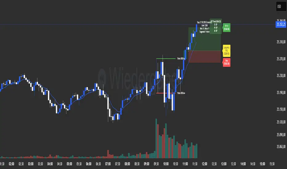
Range Bar Gaps DetectorRange Bar Gaps Detector
Overview
The Range Bar Gaps Detector identifies price gaps across multiple range bar sizes (12, 24, 60, and 120) on any trading instrument, helping traders spot potential support/resistance zones or breakout opportunities. Designed for Pine Script v6, this indicator detects gaps on range bars and exports data for use in companion scripts like Range Bar Gaps Overlap, making it ideal for multi-timeframe gap analysis.
Key Features
Multi-Range Gap Detection: Identifies gaps on 12, 24, 60, and 120-range bars, capturing both bullish (gap up) and bearish (gap down) price movements.
Customizable Sensitivity: Includes a user-defined minimum deviation (default: 10% of 14-period SMA) for 12-range gaps to filter out noise.
7-Day Lookback: Automatically prunes gaps older than 7 days to focus on recent, relevant price levels.
Data Export: Serializes up to 10 gaps per range (tops, bottoms, start bars, highest/lowest prices, and age) for seamless integration with overlap analysis scripts.
Debugging Support: Plots gap counts and aggregation data in the Data Window for easy verification of detected gaps.
How It Works
The indicator aggregates price movements to simulate higher range bars (24, 60, 120) from a base range bar chart. It detects gaps when the price jumps significantly between bars, ensuring gaps meet the minimum deviation threshold for 12-range bars. Gaps are stored in arrays, serialized for external use, and pruned after 7 days to maintain efficiency.
Usage
Add to your range bar chart (e.g., 12-range) to detect gaps across multiple ranges.
Use alongside the Range Bar Gaps Overlap indicator to visualize gaps and their overlaps as boxes on the chart.
Check the Data Window to confirm gap counts and sizes for each range (12, 24, 60, 120).
Adjust the "Minimal Deviation (%) for 12-Range" input to control gap detection sensitivity.
Settings
Minimal Deviation (%) for 12-Range: Set the minimum gap size for 12-range bars (default: 10% of 14-period SMA).
Range Sizes: Fixed at 24, 60, and 120 for higher range bar aggregation.
Notes
Ensure the script is published under your TradingView username (e.g., GreenArrow2005) for use with companion scripts.
Best used on range bar charts to maintain consistent gap detection.
For advanced overlap analysis, pair with the Range Bar Gaps Overlap indicator to highlight zones where gaps from different ranges align.
Ideal For
Traders seeking to identify key price levels for support/resistance or breakout strategies.
Multi-timeframe analysts combining gap data across various range bar sizes.
Developers building custom indicators that leverage gap data for advanced charting.
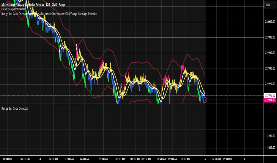
Futures Risk CalculatorFutures Risk Calculator Script - Description
The Futures Risk Calculator (FRC) is a comprehensive tool designed to help traders effectively manage risk when trading futures contracts. This script allows users to calculate risk/reward ratios directly on the chart by specifying their entry price and stop loss. It's an ideal tool for futures traders who want to quantify their potential losses and gains with precision, based on their trading account size and the number of contracts they trade.
What the Script Does:
1. Risk and Reward Calculation:
The script calculates your total risk in dollars and as a percentage of your account size based on the entry and stop-loss prices you input.
It also calculates two key levels where potential reward (Take Profit 1 and Take Profit 2) can be expected, helping you assess the reward-to-risk ratio for any trade.
2. Customizable Settings:
You can specify the size of your trading account (available $ for Futures trading) and the number of futures contracts you're trading. This allows for tailored risk management that reflects your exact trading conditions.
3. Live Chart Integration:
You add the script to your chart after opening a futures chart in TradingView. Simply click on the chart to set your Entry Price and Stop Loss. The script will instantly calculate and display the risk and reward levels based on the points you set.
Adjusting the entry and stop-loss points later is just as easy: drag and drop the levels directly on the chart, and the risk and reward calculations update automatically.
4. Futures Contract Support:
The script is pre-configured with a list of popular futures symbols (like ES, NQ, CL, GC, and more). If your preferred futures contract isn’t in the list, you can easily add it by modifying the script.
The script uses each symbol’s point value to ensure precise risk calculations, providing you with an accurate dollar risk and potential reward based on the specific contract you're trading.
How to Use the Script:
1. Apply the Script to a Futures Chart:
Open a futures contract chart in TradingView.
Add the Futures Risk Calculator (FRC) script as an indicator.
2. Set Entry and Stop Loss:
Upon applying the script, it will prompt you to select your entry price by clicking the chart where you plan to enter the market.
Next, click on the chart to set your stop-loss level.
The script will then calculate your total risk in dollars and as a percentage of your account size.
3. View Risk, Reward, and (Take Profit):
You can immediately see visual lines representing your entry, stop loss, and the calculated reward-to-risk ratio levels (Take Profit 1 and Take Profit 2).
If you want to adjust the entry or stop loss after plotting them, simply move the points on
the chart, and the script will recalculate everything for you.
4. Configure Account and Contracts:
In the script settings, you can enter your account size and adjust the number of contracts you are trading. These inputs allow the script to calculate risk in monetary terms and as a percentage, making it easier to manage your risk effectively.
5. Understand the Information in the Table:
Once you apply the script, a table will appear in the top-right corner of your chart, providing you with key information about your futures contract and the trade setup. Here's what each field represents:
Account Size: Displays your total account value, which you can set in the script's settings.
Future: Shows the selected futures symbol, along with key details such as its tick size and point value. This gives you a clear understanding of how much one point or tick is worth in dollar terms.
Entry Price: The exact price at which you plan to enter the trade, displayed in green.
Stop Loss Price: The price level where you plan to exit the trade if the market moves against you, shown in red.
Contracts: The number of futures contracts you are trading, which you can adjust in the settings.
Risk: Highlighted in orange, this field shows your total risk in dollars, as well as the percentage risk based on your account size. This is a crucial value to help you stay within your risk tolerance and manage your trades effectively.
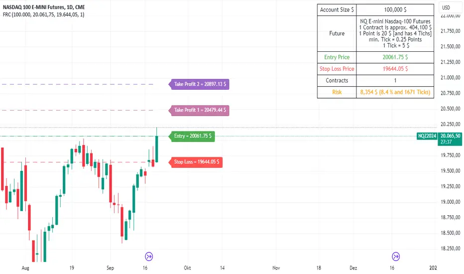
ICT Immediate Rebalance [LuxAlgo]The ICT Immediate Rebalance aims at detecting and highlighting immediate rebalances, a concept taught by Inner Circle Trader. The ICT Immediate Rebalance, although frequently overlooked, emerges as one of ICT's most influential concepts, particularly when considered within a specific context.
🔶 USAGE
Immediate rebalances, a concept taught by ICT, hold significant importance in decision-making. To comprehend the concept of immediate rebalance, it's essential to grasp the notion of the fair value gap. A fair value gap arises from market inefficiencies or imbalances, whereas an immediate rebalance leaves no gap, no inefficiencies, or no imbalances that the price would need to return to.
Following an immediate rebalance, the typical expectation is for two extension candles to ensue; failing this, the immediate rebalance is deemed unsuccessful. It's important to note that both failed and successful immediate rebalances hold significance in trading when analyzed within a contextual framework.
Immediate rebalances can manifest across various locations and timeframes. It's recommended to analyze them in conjunction with other ICT tools or technical indicators to gain a more comprehensive understanding of market dynamics.
🔹 Multi Timeframe
The script facilitates multi-timeframe analysis, enabling users to display immediate rebalances from higher timeframes.
Enabling the display of higher timeframe candles helps visualize the detected immediate rebalance patterns.
🔹 Dashboard
The dashboard offers statistical insights into immediate rebalances.
🔶 SETTINGS
🔹 Immediate Rebalances
Timeframe: this option is to identify immediate rebalances from higher timeframes. If a timeframe lower than the chart's timeframe is selected, calculations will be based on the chart's timeframe.
Bullish, and Bearish Immediate Rebalances: color customization options.
Wicks 75%, %50, and %25: color customization options of the wick price levels for the detected immediate rebalances.
Immediate Rebalance Candles: toggles the visualization of higher timeframe candles where immediate rebalance is detected.
Confirmation (Bars): specifies the number of bars required to confirm the validation of the detected immediate rebalance.
Immediate Rebalance Icon: allows customization of the size of the icon used to represent the immediate rebalance.
🔹 Dashboard
Dashboard: toggles the visualization of the dashboard, sets its location, and customizes the size of the dashboard.
🔶 RELATED SCRIPTS
Fair-Value-Gap
Thanks to our community for recommending this script. For more conceptual scripts and related content, we welcome you to explore by visiting >>> LuxAlgo-Scripts .
Pro Trading Art - Head And ShouldersHow the Script Works:
1. The script identifies potential Head and Shoulders patterns by searching for specific pivot highs and pivot lows in the price data.
2. It checks for the presence of a left shoulder, head, and right shoulder based on the conditions defined in the script.
3. If a valid Head and Shoulders pattern is found, the script plots lines and labels on the chart to visualize the pattern.
4. The script also identifies Inverted Head and Shoulders patterns using similar logic but with different conditions.
5. It plots lines and labels for the Inverted Head and Shoulders pattern.
6. The script generates short and long conditions based on the patterns. Short conditions trigger when the close price crosses below the neck level of a Head and Shoulders pattern, while long conditions trigger when the close price crosses above the neck level of an Inverted Head and Shoulders pattern.
7. It plots sell and buy signal shapes on the chart when the short and long conditions are met, respectively.
8. The script can also trigger alerts to notify the user when a valid Head and Shoulders or Inverted Head and Shoulders pattern is detected.
9. The script provides visual cues on the chart to help users identify potential trading opportunities.
10. The logic and parameters of the script can be modified by the user to customize the behavior and adapt it to different trading strategies.
How Users Can Make Profit Using This Script:
1. Identify potential short-selling opportunities: When a valid Head and Shoulders pattern is detected and a short condition is met, it indicates a potential trend reversal. Traders can consider opening short positions to profit from a downward price movement.
2. Identify potential long-buying opportunities: When a valid Inverted Head and Shoulders pattern is detected and a long condition is met, it suggests a potential trend reversal. Traders can consider opening long positions to profit from an upward price movement.
3. Combine with additional analysis: Users can utilize this script as a tool in their overall trading strategy. They can combine the signals generated by the script with other technical indicators, fundamental analysis, or market sentiment to make more informed trading decisions.
4. Define appropriate entry and exit points: Traders can use the lines and labels plotted by the script to determine entry and exit points for their trades. For example, they may choose to enter a short position after the price crosses below the neck level and exit when the price reaches a predetermined target or when the pattern is invalidated.
5. Set risk management measures: It is important for users to implement proper risk management strategies when trading based on the script's signals. They should define stop-loss orders to limit potential losses if the trade goes against them and consider setting profit targets to secure profits when the trade moves in their favor.

Intrabar Efficiency Ratio█ OVERVIEW
This indicator displays a directional variant of Perry Kaufman's Efficiency Ratio, designed to gauge the "efficiency" of intrabar price movement by comparing the sum of movements of the lower timeframe bars composing a chart bar with the respective bar's movement on an average basis.
█ CONCEPTS
Efficiency Ratio (ER)
Efficiency Ratio was first introduced by Perry Kaufman in his 1995 book, titled "Smarter Trading". It is the ratio of absolute price change to the sum of absolute changes on each bar over a period. This tells us how strong the period's trend is relative to the underlying noise. Simply put, it's a measure of price movement efficiency. This ratio is the modulator utilized in Kaufman's Adaptive Moving Average (KAMA), which is essentially an Exponential Moving Average (EMA) that adapts its responsiveness to movement efficiency.
ER's output is bounded between 0 and 1. A value of 0 indicates that the starting price equals the ending price for the period, which suggests that price movement was maximally inefficient. A value of 1 indicates that price had travelled no more than the distance between the starting price and the ending price for the period, which suggests that price movement was maximally efficient. A value between 0 and 1 indicates that price had travelled a distance greater than the distance between the starting price and the ending price for the period. In other words, some degree of noise was present which resulted in reduced efficiency over the period.
As an example, let's say that the price of an asset had moved from $15 to $14 by the end of a period, but the sum of absolute changes for each bar of data was $4. ER would be calculated like so:
ER = abs(14 - 15)/4 = 0.25
This suggests that the trend was only 25% efficient over the period, as the total distanced travelled by price was four times what was required to achieve the change over the period.
Intrabars
Intrabars are chart bars at a lower timeframe than the chart's. Each 1H chart bar of a 24x7 market will, for example, usually contain 60 intrabars at the LTF of 1min, provided there was market activity during each minute of the hour. Mining information from intrabars can be useful in that it offers traders visibility on the activity inside a chart bar.
Lower timeframes (LTFs)
A lower timeframe is a timeframe that is smaller than the chart's timeframe. This script determines which LTF to use by examining the chart's timeframe. The LTF determines how many intrabars are examined for each chart bar; the lower the timeframe, the more intrabars are analyzed, but fewer chart bars can display indicator information because there is a limit to the total number of intrabars that can be analyzed.
Intrabar precision
The precision of calculations increases with the number of intrabars analyzed for each chart bar. As there is a 100K limit to the number of intrabars that can be analyzed by a script, a trade-off occurs between the number of intrabars analyzed per chart bar and the chart bars for which calculations are possible.
Intrabar Efficiency Ratio (IER)
Intrabar Efficiency Ratio applies the concept of ER on an intrabar level. Rather than comparing the overall change to the sum of bar changes for the current chart's timeframe over a period, IER compares single bar changes for the current chart's timeframe to the sum of absolute intrabar changes, then applies smoothing to the result. This gives an indication of how efficient changes are on the current chart's timeframe for each bar of data relative to LTF bar changes on an average basis. Unlike the standard ER calculation, we've opted to preserve directional information by not taking the absolute value of overall change, thus allowing it to be utilized as a momentum oscillator. However, by taking the absolute value of this oscillator, it could potentially serve as a replacement for ER in the design of adaptive moving averages.
Since this indicator preserves directional information, IER can be regarded as similar to the Chande Momentum Oscillator (CMO) , which was presented in 1994 by Tushar Chande in "The New Technical Trader". Both CMO and ER essentially measure the same relationship between trend and noise. CMO simply differs in scale, and considers the direction of overall changes.
█ FEATURES
Display
Three different display types are included within the script:
• Line : Displays the middle length MA of the IER as a line .
Color for this display can be customized via the "Line" portion of the "Visuals" section in the script settings.
• Candles : Displays the non-smooth IER and two moving averages of different lengths as candles .
The `open` and `close` of the candle are the longest and shortest length MAs of the IER respectively.
The `high` and `low` of the candle are the max and min of the IER, longest length MA of the IER, and shortest length MA of the IER respectively.
Colors for this display can be customized via the "Candles" portion of the "Visuals" section in the script settings.
• Circles : Displays three MAs of the IER as circles .
The color of each plot depends on the percent rank of the respective MA over the previous 100 bars.
Different colors are triggered when ranks are below 10%, between 10% and 50%, between 50% and 90%, and above 90%.
Colors for this display can be customized via the "Circles" portion of the "Visuals" section in the script settings.
With either display type, an optional information box can be displayed. This box shows the LTF that the script is using, the average number of lower timeframe bars per chart bar, and the number of chart bars that contain LTF data.
Specifying intrabar precision
Ten options are included in the script to control the number of intrabars used per chart bar for calculations. The greater the number of intrabars per chart bar, the fewer chart bars can be analyzed.
The first five options allow users to specify the approximate amount of chart bars to be covered:
• Least Precise (Most chart bars) : Covers all chart bars by dividing the current timeframe by four.
This ensures the highest level of intrabar precision while achieving complete coverage for the dataset.
• Less Precise (Some chart bars) & More Precise (Less chart bars) : These options calculate a stepped LTF in relation to the current chart's timeframe.
• Very precise (2min intrabars) : Uses the second highest quantity of intrabars possible with the 2min LTF.
• Most precise (1min intrabars) : Uses the maximum quantity of intrabars possible with the 1min LTF.
The stepped lower timeframe for "Less Precise" and "More Precise" options is calculated from the current chart's timeframe as follows:
Chart Timeframe Lower Timeframe
Less Precise More Precise
< 1hr 1min 1min
< 1D 15min 1min
< 1W 2hr 30min
> 1W 1D 60min
The last five options allow users to specify an approximate fixed number of intrabars to analyze per chart bar. The available choices are 12, 24, 50, 100, and 250. The script will calculate the LTF which most closely approximates the specified number of intrabars per chart bar. Keep in mind that due to factors such as the length of a ticker's sessions and rounding of the LTF, it is not always possible to produce the exact number specified. However, the script will do its best to get as close to the value as possible.
Specifying MA type
Seven MA types are included in the script for different averaging effects:
• Simple
• Exponential
• Wilder (RMA)
• Weighted
• Volume-Weighted
• Arnaud Legoux with `offset` and `sigma` set to 0.85 and 6 respectively.
• Hull
Weighting
This script includes the option to weight IER values based on the percent rank of absolute price changes on the current chart's timeframe over a specified period, which can be enabled by checking the "Weigh using relative close changes" option in the script settings. This places reduced emphasis on IER values from smaller changes, which may help to reduce noise in the output.
█ FOR Pine Script™ CODERS
• This script imports the recently published lower_ltf library for calculating intrabar statistics and the optimal lower timeframe in relation to the current chart's timeframe.
• This script uses the recently released request.security_lower_tf() Pine Script™ function discussed in this blog post .
It works differently from the usual request.security() in that it can only be used on LTFs, and it returns an array containing one value per intrabar.
This makes it much easier for programmers to access intrabar information.
• This script implements a new recommended best practice for tables which works faster and reduces memory consumption.
Using this new method, tables are declared only once with var , as usual. Then, on the first bar only, we use table.cell() to populate the table.
Finally, table.set_*() functions are used to update attributes of table cells on the last bar of the dataset.
This greatly reduces the resources required to render tables.
Look first. Then leap.

Matrix Library (Linear Algebra, incl Multiple Linear Regression)What's this all about?
Ever since 1D arrays were added to Pine Script, many wonderful new opportunities have opened up. There has been a few implementations of matrices and matrix math (most notably by TradingView-user tbiktag in his recent Moving Regression script: ). However, so far, no comprehensive libraries for matrix math and linear algebra has been developed. This script aims to change that.
I'm not math expert, but I like learning new things, so I took it upon myself to relearn linear algebra these past few months, and create a matrix math library for Pine Script. The goal with the library was to make a comprehensive collection of functions that can be used to perform as many of the standard operations on matrices as possible, and to implement functions to solve systems of linear equations. The library implements matrices using arrays, and many standard functions to manipulate these matrices have been added as well.
The main purpose of the library is to give users the ability to solve systems of linear equations (useful for Multiple Linear Regression with K number of independent variables for example), but it can also be used to simulate 2D arrays for any purpose.
So how do I use this thing?
Personally, what I do with my private Pine Script libraries is I keep them stored as text-files in a Libraries folder, and I copy and paste them into my code when I need them. This library is quite large, so I have made sure to use brackets in comments to easily hide any part of the code. This helps with big libraries like this one.
The parts of this script that you need to copy are labeled "MathLib", "ArrayLib", and "MatrixLib". The matrix library is dependent on the functions from these other two libraries, but they are stripped down to only include the functions used by the MatrixLib library.
When you have the code in your script (pasted somewhere below the "study()" call), you can create a matrix by calling one of the constructor functions. All functions in this library start with "matrix_", and all constructors start with either "create" or "copy". I suggest you read through the code though. The functions have very descriptive names, and a short description of what each function does is included in a header comment directly above it. The functions generally come in the following order:
Constructors: These are used to create matrices (empy with no rows or columns, set shape filled with 0s, from a time series or an array, and so on).
Getters and setters: These are used to get data from a matrix (like the value of an element or a full row or column).
Matrix manipulations: These functions manipulate the matrix in some way (for example, functions to append columns or rows to a matrix).
Matrix operations: These are the matrix operations. They include things like basic math operations for two indices, to transposing a matrix.
Decompositions and solvers: Next up are functions to solve systems of linear equations. These include LU and QR decomposition and solvers, and functions for calculating the pseudo-inverse or inverse of a matrix.
Multiple Linear Regression: Lastly, we find an implementation of a multiple linear regression, including all the standard statistics one can expect to find in most statistical software packages.
Are there any working examples of how to use the library?
Yes, at the very end of the script, there is an example that plots the predictions from a multiple linear regression with two independent (explanatory) X variables, regressing the chart data (the Y variable) on these X variables. You can look at this code to see a real-world example of how to use the code in this library.
Are there any limitations?
There are no hard limiations, but the matrices uses arrays, so the number of elements can never exceed the number of elements supported by Pine Script (minus 2, since two elements are used internally by the library to store row and column count). Some of the operations do use a lot of resources though, and as a result, some things can not be done without timing out. This can vary from time to time as well, as this is primarily dependent on the available resources from the Pine Script servers. For instance, the multiple linear regression cannot be used with a lookback window above 10 or 12 most of the time, if the statistics are reported. If no statistics are reported (and therefore not calculated), the lookback window can usually be extended to around 60-80 bars before the servers time out the execution.
Hopefully the dev-team at TradingView sees this script and find ways to implement this functionality diretly into Pine Script, as that would speed up many of the operations and make things like MLR (multiple linear regression) possible on a bigger lookback window.
Some parting words
This library has taken a few months to write, and I have taken all the steps I can think of to test it for bugs. Some may have slipped through anyway, so please let me know if you find any, and I'll try my best to fix them when I have time to do so. This library is intended to help the community. Therefore, I am releasing the library as open source, in the hopes that people may improving on it, or using it in their own work. If you do make something cool with this, or if you find ways to improve the code, please let me know in the comments.

[PX] External LevelHello everyone,
today I'd like to share a script, which enables you to use external logic to plot levels on your chart.
How does it work?
The concept is based on two scripts. One script, which uses an external input as a trigger to print a new level and one script that calculates an output, which will be fetched.
Sounds complicated? It really is not! Let's take a closer look.
// This source code is subject to the terms of the Mozilla Public License 2.0 at mozilla.org
// © paaax
//@version=4
study("RSI OS/OB")
l = input(14, "RSI Length")
ob = input(70, "Overbought")
os = input(30, "Oversold")
r = rsi(close, l)
hline(ob)
hline(os)
plot(r, "RSI", color=color.orange)
// The following plot produces an output, which will be fetched the "External Level"-script.
// It evaluates to one of the following three values: 1.0, -1.0 or 0.0
plot(crossover(r, ob) ? 1.0 : crossunder(r, os) ? -1.0 : 0.0, "Output", transp=100)
The example script above uses an RSI and two threshold levels (70 and 30). The logic here is, that whenever the RSI is crossing down the lower threshold or crossing up the upper threshold we'd consider the current movement to be either oversold or overbought. Therefore, it's a point of interest, which we could visualize with a level.
The script creates an output when the crossover or crossunder of a threshold happens. A crossover would result in a value of 1.0, a crossunder in a value of -1.0. In all other cases the value would be 0.0.
The output of the RSI script would then be used as an input of the External Level script, which has a "Source"-parameter in its input-section. If the fetched input shows 1.0, then the script prints a resistance level. If it shows -1.0 a support level will be printed. And that's basically it. A very simple approach to print levels on your chart with an infinite number of use cases.
For example, you could use fetch outputs from a MACD script, MA script, outputs based on volume or price movement. Just remember the output has to evaluate to either 1.0 or -1.0 and has to be selected in the input-section.
Hope that might be useful to some of you :)
Please click the "Like"-button and follow me for future open-source script publications.
If you are looking for help with your custom PineScript development, don't hesitate to contact me directly here on Tradingview or through the link in my signature :)