HTF Frequency Zone [BigBeluga]🔵 OVERVIEW
HTF Frequency Zone highlights the dominant price level (Point of Control) and the full high–low expansion of any higher timeframe — Daily, Weekly, or Monthly. It captures the frequency of closes inside each HTF candle and plots the most traded “frequency zone”, allowing traders to easily see where price spent the most time and where buy/sell pressure accumulated.
This tool transforms each higher-timeframe bar into a fully visualized structure:
• Top = HTF high
• Bottom = HTF low
• Midline = HTF Frequency POC
• Color-coded zones = bullish or bearish bias
• Labels = counts of bullish and bearish candles inside the HTF range
It is designed to give traders an immediate understanding of high-timeframe balance, imbalance, and price attraction zones.
🔵 CONCEPTS
HTF Partitioning — Each Weekly/Daily/Monthly candle is converted into a dedicated zone with its own High, Low, and Frequency Point of Control.
Frequency POC (Most Touched Price) — The indicator divides the HTF range into 100 bins and counts how many times price closed near each level.
Dominant Zone — The level with the highest frequency becomes the HTF “Value Zone,” plotted as a bold central line.
Directional Bias —
• Bullish HTF zone
• Bearish HTF zone
Internal Candle Counting — Within each HTF period the indicator counts:
• Buy candles (close > open)
• Sell candles (close < open)
This reveals whether intraperiod flow was bullish or bearish.
HTF Structure Blocks — High, Low, and POC are connected across the entire higher-timeframe duration, showing the real shape of HTF balance.
🔵 FEATURES
Automatic HTF Zone Construction — Generates a complete price zone every time the selected timeframe flips (Daily / Weekly / Monthly).
Dynamic High & Low Extraction — The indicator scans every bar inside the HTF window to find true extremes of the range.
100-Level Frequency Scan — Each close within the period is assigned to a bin, creating a detailed distribution of price interaction.
HTF POC Highlighting — The most frequent price level is plotted with a bold red line for immediate visual clarity.
Bull/Bear Coloring —
• Green → Bullish HTF zone.
• Orange → Bearish HTF zone.
Zone Shading — High–Low range is filled with a semi-transparent color matching trend direction.
Buy/Sell Candle Counters — Printed at the top and bottom of each HTF block, showing how many internal candles were bullish or bearish.
POC Label — Displays frequency count (how many touches) at the POC level.
Adaptive Threshold Warning — If bars inside the HTF window are too few (<10), the indicator warns the trader to switch timeframe.
🔵 HOW TO USE
Higher-Timeframe Biasing — Read the zone color to determine if the HTF candle leaned bullish or bearish.
Value Zone Reactions — Price often reacts to the Frequency POC; use it as support/resistance or liquidity magnet.
Range Context — Identify when price is trading near HTF highs (breakout potential) or lows (reversal potential).
Momentum Evaluation — More bullish internal candles = internal buying pressure; more bearish = internal selling pressure.
Swing Trading — Use HTF zones as the “macro map,” then execute trades on lower timeframes aligned with the zone structure.
Liquidity Awareness — The HTF POC often aligns with algorithmic liquidity levels, making it a strong reaction point.
🔵 CONCLUSION
HTF Frequency Zone transforms raw higher-timeframe candles into detailed distribution zones that reveal true market behavior inside the HTF structure. By showing highs, lows, buying/selling activity, and the most interacted price level (Frequency POC), this tool becomes invaluable for traders who want to align executions with powerful HTF levels, liquidity magnets, and structural zones.
Frequency

[iQ]PRO Volume Frequency Profile+++🌌 PRO Volume Frequency Profile+++: The Fusion of Precision and Market Flow
The PRO Volume Frequency Profile+++ ( PRO VFP+++) is a next-generation analytical instrument designed for the discerning professional trader. It masterfully synthesizes multiple advanced concepts—Dynamic Linear Regression, High-Fidelity Frequency Analysis, and a Volumetric Distribution Profile—into a single, unified view of market structure. This powerful fusion provides unparalleled context for identifying high-probability turning points and key areas of interest.
🔬 Core Innovation: The Symbiotic Market Model
At its heart, the PRO VFP+++ is built on a proprietary methodology that transcends traditional price action by analyzing the frequency and distribution of traded volume relative to the dominant price trend.
Adaptive Regression Channel: The indicator establishes a highly dynamic Linear Regression channel, which acts as the core gravity well of the current trend. This channel is then protected by multi-tier Standard Deviation (SD) Bands with highly optimized, non-standard multipliers, defining the boundaries of expected price movement.
High-Resolution Frequency Bands: An integrated, proprietary Frequency Analysis component detects the underlying rhythmic oscillation in the market. This mechanism generates Frequency Bands that fluctuate around the core regression line, providing an exceptionally sensitive, leading, and dynamic channel for short-term mean-reversion and continuation signals.
Volumetric Profile Insight: A sophisticated Volume Frequency Profile is meticulously constructed over the look back period defined by the Linear Regression. This profile maps the distribution of trading activity, with an advanced implementation that provides a directional bias (Buy/Sell color gradient) within the volume nodes themselves, offering a deeper understanding of market participation.
✨ The Edge: Strategic Node Detection
The indicator's most compelling feature is its Intelligent Node Detection System. This system is specifically engineered to filter out market noise and highlight critical confluence zones:
Confluence Nodes: Automatically identifies and marks prices where the statistically significant Volume Nodes from the profile interact with the calculated Linear Regression lines and Standard Deviation Bands. These intersection points are areas where technical structure and realized market flow align, signaling price magnets or potential reversal zones.
Customizable Sensitivity: The system is governed by a Node Sensitivity parameter, allowing the user to fine-tune the filter for market conditions, ensuring only the most robust interactions are flagged.
🚨 Real-Time Opportunity & Security
To ensure maximum efficiency, the PRO VFP+++ features comprehensive, real-time Alerts based on all three core components:
Significant Node Cross: Alerts when price intersects a high-confluence interaction node.
Regression Line Touch: Alerts when price tests the core regression line, indicating a re-test of the dominant trend.
SD Band Touch: Alerts upon contact with the statistical boundaries, signaling potential overextension or trend strength.
This is a professional-grade, proprietary instrument. The source code is intentionally closed and protected to preserve the unique advantage of its underlying algorithms, which are the result of extensive research and optimization. Access is restricted and may be limited to invited, paying members only.
Unlock the next level of market structure analysis with the PRO VFP+++.

Frequency Momentum Oscillator [QuantAlgo]🟢 Overview
The Frequency Momentum Oscillator applies Fourier-based spectral analysis principles to price action to identify regime shifts and directional momentum. It calculates Fourier coefficients for selected harmonic frequencies on detrended price data, then measures the distribution of power across low, mid, and high frequency bands to distinguish between persistent directional trends and transient market noise. This approach provides traders with a quantitative framework for assessing whether current price action represents meaningful momentum or merely random fluctuations, enabling more informed entry and exit decisions across various asset classes and timeframes.
🟢 How It Works
The calculation process removes the dominant trend from price data by subtracting a simple moving average, isolating cyclical components for frequency analysis:
detrendedPrice = close - ta.sma(close , frequencyPeriod)
The detrended price series undergoes frequency decomposition through Fourier coefficient calculation across the first 8 harmonics. For each harmonic frequency, the algorithm computes sine and cosine components across the lookback window, then derives power as the sum of squared coefficients:
for k = 1 to 8
cosSum = 0.0
sinSum = 0.0
for n = 0 to frequencyPeriod - 1
angle = 2 * math.pi * k * n / frequencyPeriod
cosSum := cosSum + detrendedPrice * math.cos(angle)
sinSum := sinSum + detrendedPrice * math.sin(angle)
power = (cosSum * cosSum + sinSum * sinSum) / frequencyPeriod
Power measurements are aggregated into three frequency bands: low frequencies (harmonics 1-2) capturing persistent cycles, mid frequencies (harmonics 3-4), and high frequencies (harmonics 5-8) representing noise. Each band's power normalizes against total spectral power to create percentage distributions:
lowFreqNorm = totalPower > 0 ? (lowFreqPower / totalPower) * 100 : 33.33
highFreqNorm = totalPower > 0 ? (highFreqPower / totalPower) * 100 : 33.33
The normalized frequency components undergo exponential smoothing before calculating spectral balance as the difference between low and high frequency power:
smoothLow = ta.ema(lowFreqNorm, smoothingPeriod)
smoothHigh = ta.ema(highFreqNorm, smoothingPeriod)
spectralBalance = smoothLow - smoothHigh
Spectral balance combines with price momentum through directional multiplication, producing a composite signal that integrates frequency characteristics with price direction:
momentum = ta.change(close , frequencyPeriod/2)
compositeSignal = spectralBalance * math.sign(momentum)
finalSignal = ta.ema(compositeSignal, smoothingPeriod)
The final signal oscillates around zero, with positive values indicating low-frequency dominance coupled with upward momentum (trending up), and negative values indicating either high-frequency dominance (choppy market) or downward momentum (trending down).
🟢 How to Use This Indicator
→ Long/Short Signals: the indicator generates long signals when the smoothed composite signal crosses above zero (indicating low-frequency directional strength dominates) and short signals when it crosses below zero (indicating bearish momentum persistence).
→ Upper and Lower Reference Lines: the +25 and -25 reference lines serve as threshold markers for momentum strength. Readings beyond these levels indicate strong directional conviction, while oscillations between them suggest consolidation or weakening momentum. These references help traders distinguish between strong trending regimes and choppy transitional periods.
→ Preconfigured Presets: three optimized configurations are available with Default (32, 3) offering balanced responsiveness, Fast Response (24, 2) designed for scalping and intraday trading, and Smooth Trend (40, 5) calibrated for swing trading and position trading with enhanced noise filtration.
→ Built-in Alerts: the indicator includes three alert conditions for automated monitoring - Long Signal (momentum shifts bullish), Short Signal (momentum shifts bearish), and Signal Change (any directional transition). These alerts enable traders to receive real-time notifications without continuous chart monitoring.
→ Color Customization: four visual themes (Classic green/red, Aqua blue/orange, Cosmic aqua/purple, Custom) allow chart customization for different display environments and personal preferences.

Count█ OVERVIEW
A library of functions for counting the number of times (frequency) that elements occur in an array or matrix.
█ USAGE
Import the Count library.
import joebaus/count/1 as c
Create an array or matrix that is a `float`, `int`, `string`, or `bool` type to count elements from, then call the count function on the array or matrix.
id = array.from(1.00, 1.50, 1.25, 1.00, 0.75, 1.25, 1.75, 1.25)
countMap = id.count() // Alternatively: countMap = c.count(id)
The "count map" will return a map with keys for each unique element in the array or matrix, and with respective values representing the number of times the unique element was counted. The keys will be the same type as the array or matrix counted. The values will always be an `int` type.
array mapKeys = countMap.keys() // Returns unique keys
array mapValues = countMap.values() // Returns counts
If an array is in ascending or descending order, then the keys of the map will also generate in the same order.
intArray = array.from(2, 2, 2, 3, 4, 4, 4, 4, 4, 6, 6) // Ascending order
map countMap = intArray.count() // Creates a "count map" of all unique elements
array mapKeys = countMap.keys() // Returns // Ascending order
array mapValues = countMap.values() // Returns count
Include a value to get the count of only that value in an array or matrix.
floatMatrix = matrix.new(3, 3, 0.0)
floatMatrix.set(0, 0, 1.0), floatMatrix.set(1, 0, 1.0), floatMatrix.set(2, 0, 1.0)
floatMatrix.set(0, 1, 1.5), floatMatrix.set(1, 1, 2.0), floatMatrix.set(2, 1, 2.5)
floatMatrix.set(0, 2, 1.0), floatMatrix.set(1, 2, 2.5), floatMatrix.set(2, 2, 1.5)
int countFloatMatrix = floatMatrix.count(1.0) // Counts all 1.0 elements, returns 5
// Alternatively: int countFloatMatrix = c.count(floatMatrix, 1.0)
The string method of count() can use strings or regular expressions like "bull*" to count all matching occurrences in a string array.
stringArray = array.from('bullish', 'bull', 'bullish', 'bear', 'bull', 'bearish', 'bearish')
int countString = stringArray.count('bullish') // Returns 2
int countStringRegex = stringArray.count('bull*') // Returns 4
To count multiple values, use an array of values instead of a single value. Returning a count map only of elements in the array.
countArray = array.from(1.0, 2.5)
map countMap = floatMatrix.count(countArray)
array mapKeys = countMap.keys() // Returns keys
array mapValues = countMap.values() // Returns counts
Multiple regex patterns or strings can be counted as well.
stringMatrix = matrix.new(3, 3, '')
stringMatrix.set(0, 0, 'a'), stringMatrix.set(1, 0, 'a'), stringMatrix.set(2, 0, 'a')
stringMatrix.set(0, 1, 'b'), stringMatrix.set(1, 1, 'c'), stringMatrix.set(2, 1, 'd')
stringMatrix.set(0, 2, 'a'), stringMatrix.set(1, 2, 'd'), stringMatrix.set(2, 2, 'b')
// Count the number of times the regex patterns `'^(a|c)$'` and `'^(b|d)$'` occur
array regexes = array.from('^(a|c)$', '^(b|d)$')
map countMap = stringMatrix.count(regexes)
array mapKeys = countMap.keys() // Returns
array mapValues = countMap.values() // Returns
An optional comparison operator can be specified to count the number of times an equality was satisfied for `float`, `int`, and `bool` methods of `count()`.
intArray = array.from(2, 2, 2, 3, 4, 4, 4, 4, 4, 6, 6)
// Count the number of times an element is greater than 4
countInt = intArray.count(4, '>') // Returns 2
When passing an array of values to count and a comparison operator, the operator will apply to each value.
intArray = array.from(2, 2, 2, 3, 4, 4, 4, 4, 4, 6, 6)
values = array.from(3, 4)
// Count the number of times and element is greater than 3 and 4
map countMap = intArray.count(values, '>')
array mapKeys = countMap.keys() // Returns
array mapValues = countMap.values() // Returns
Multiple comparison operators can be applied when counting multiple values.
intMatrix = matrix.new(3, 3, 0)
intMatrix.set(0, 0, 2), intMatrix.set(1, 0, 3), intMatrix.set(2, 0, 5)
intMatrix.set(0, 1, 2), intMatrix.set(1, 1, 4), intMatrix.set(2, 1, 2)
intMatrix.set(0, 2, 5), intMatrix.set(1, 2, 2), intMatrix.set(2, 2, 3)
values = array.from(3, 4)
comparisons = array.from('<', '>')
// Count the number of times an element is less than 3 and greater than 4
map countMap = intMatrix.count(values, comparisons)
array mapKeys = countMap.keys() // Returns
array mapValues = countMap.values() // Returns

Deviation Trend Profile [BigBeluga]🔵 OVERVIEW
A statistical trend analysis tool that combines moving average dynamics with standard deviation zones and trend-specific price distribution.
This is an experimental indicator designed for educational and learning purposes only.
🔵 CONCEPTS
Trend Detection via SMA Slope: Detects trend shifts when the slope of the SMA exceeds a ±0.1 threshold.
Standard Deviation Zones: Calculates ±1, ±2, and ±3 levels from the SMA using ATR, forming dynamic envelopes around the mean.
Trend Distribution Profile: Builds a histogram that shows how often price closed within each deviation zone during the active trend phase.
🔵 FEATURES
Trend Signals: Immediate shift markers using colored circles at trend reversals.
SMA Gradient Coloring: The SMA line dynamically changes color based on its directional slope.
Trend Duration Label: A label above the histogram shows how many bars the current trend has lasted.
Trend Distribution Histogram: Visual bin-based profile showing frequency of price closes within deviation bands during trend lookback period.
Adjustable Bin Count: Set the granularity of the distribution using the “Bins Amount” input.
Deviation Labels and Zones: Clearly marked ±1, ±2, ±3 lines with consistent color scheme.
Trend Strength Insight:
• Wide profile skewed to ±2/3 = strong directional trend.
• Profile clustered near SMA = potential trend exhaustion or range.
🔵 HOW TO USE
Use trend shift dots as entry signals:
• 🔵 = Bullish start
• 🔴 = Bearish start
Trade with the trend when price clusters in outer zones (±2 or ±3).
Be cautious or fade the trend when price distribution contracts toward the SMA.
View across multiple timeframes for trend confluence or divergence.
🔵 CONCLUSION
Deviation Trend Profile visualizes how price distributes during trends relative to statistical deviation zones.
It’s a powerful confluence tool for identifying strength, exhaustion, and the rhythm of price behavior—ideal for swing traders and volatility analysts alike.

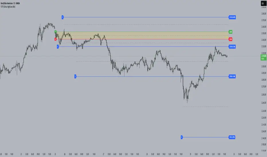
Cycle Theory + Frequency TheoryCycle Theory attempts to predict, through volatility, support/resistance points where the market may reach/reverse a trend. This theory's calculation is based on a reference candle that the user chooses, usually the first candle of the day/week's session. From this point on, if the level is broken upwards or downwards, the 1st Cycle begins with the same distance between the high/low or open/close of the reference candle. From the 2nd Cycle onwards, the size becomes the sum of all the last cycles formed, and so on.
Frequency Theory is similar, but its levels always have the same size as the high/low or open/close of the reference candle.
Adaptive Resonance Oscillator [AlgoAlpha]Introducing the Adaptive Resonance Oscillator , an advanced momentum-based oscillator designed to dynamically adjust to changing market conditions. This innovative indicator detects market frequency through a Hilbert Transform approach, adapting in real-time to identify overbought and oversold conditions with improved accuracy. With built-in divergence detection, trend analysis, and customizable smoothing, this tool is perfect for traders looking to refine their entries and exits based on adaptive oscillation mechanics.
🚀 Key Features :
🔹 Adaptive Frequency Detection – Uses Hilbert Transform principles to dynamically determine market cycle length for precise oscillator calculation.
⚙️ Customizable Smoothing – Option to apply a Hull Moving Average (HMA) for enhanced signal clarity.
📈 Divergence Detection – Identifies bullish and bearish divergences with visual markers, helping traders spot early trend reversals.
🟢 Overbought & Oversold Signals – Highlights extreme momentum conditions with adjustable thresholds.
🔔 Real-Time Alerts – Get notified for crossovers, divergences, and strong trend shifts directly on your TradingView chart.
🎨 Fully Customizable Appearance – Modify colors, divergence sensitivity, and smoothing options to fit your trading style.
🛠 How to Use :
Add the Adaptive Resonance Oscillator to your TradingView chart by clicking the ★ to favorite it.
Monitor the Charts , switch between smoothed and I smoothed modes to identify trend and price swings, use divergences and reversal signals for potential entry/exits.
Set alerts for bullish/bearish crossovers and divergence signals to stay ahead of market moves.
⚙ How It Works :
The indicator begins by applying a Hilbert Transform frequency estimation to the price series, identifying the dominant market cycle length. This is used to calculate a period for the RSI that matches its resonant frequency with the dominant market frequency, dynamically adjusting the Oscillator. The oscillator then applies an optional Hull Moving Average (HMA) smoothing for signal refinement. Additionally, the indicator scans for bullish and bearish divergences by comparing oscillator movements against price action, plotting signals accordingly. When overbought/oversold conditions or divergence events occur, alerts are triggered to notify the trader in real time.

High/Low Location Frequency [LuxAlgo]The High/Low Location Frequency tool provides users with probabilities of tops and bottoms at user-defined periods, along with advanced filters that offer deep and objective market information about the likelihood of a top or bottom in the market.
🔶 USAGE
There are four different time periods that traders can select for analysis of probabilities:
HOUR OF DAY: Probability of occurrence of top and bottom prices for each hour of the day
DAY OF WEEK: Probability of occurrence of top and bottom prices for each day of the week
DAY OF MONTH: Probability of occurrence of top and bottom prices for each day of the month
MONTH OF YEAR: Probability of occurrence of top and bottom prices for each month
The data is displayed as a dashboard, which users can position according to their preferences. The dashboard includes useful information in the header, such as the number of periods and the date from which the data is gathered. Additionally, users can enable active filters to customize their view. The probabilities are displayed in one, two, or three columns, depending on the number of elements.
🔹 Advanced Filters
Advanced Filters allow traders to exclude specific data from the results. They can choose to use none or all filters simultaneously, inputting a list of numbers separated by spaces or commas. However, it is not possible to use both separators on the same filter.
The tool is equipped with five advanced filters:
HOURS OF DAY: The permitted range is from 0 to 23.
DAYS OF WEEK: The permitted range is from 1 to 7.
DAYS OF MONTH: The permitted range is from 1 to 31.
MONTHS: The permitted range is from 1 to 12.
YEARS: The permitted range is from 1000 to 2999.
It should be noted that the DAYS OF WEEK advanced filter has been designed for use with tickers that trade every day, such as those trading in the crypto market. In such cases, the numbers displayed will range from 1 (Sunday) to 7 (Saturday). Conversely, for tickers that do not trade over the weekend, the numbers will range from 1 (Monday) to 5 (Friday).
To illustrate the application of this filter, we will exclude results for Mondays and Tuesdays, the first five days of each month, January and February, and the years 2020, 2021, and 2022. Let us review the results:
DAYS OF WEEK: `2,3` or `2 3` (for crypto) or `1,2` or `1 2` (for the rest)
DAYS OF MONTH: `1,2,3,4,5` or `1 2 3 4 5`
MONTHS: `1,2` or `1 2`
YEARS: `2020,2021,2022` or `2020 2021 2022`
🔹 High Probability Lines
The tool enables traders to identify the next period with the highest probability of a top (red) and/or bottom (green) on the chart, marked with two horizontal lines indicating the location of these periods.
🔹 Top/Bottom Labels and Periods Highlight
The tool is capable of indicating on the chart the upper and lower limits of each selected period, as well as the commencement of each new period, thus providing traders with a convenient reference point.
🔶 SETTINGS
Period: Select how many bars (hours, days, or months) will be used to gather data from, max value as default.
Execution Window: Select how many bars (hours, days, or months) will be used to gather data from
🔹 Advanced Filters
Hours of day: Filter which hours of the day are excluded from the data, it accepts a list of hours from 0 to 23 separated by commas or spaces, users can not mix commas or spaces as a separator, must choose one
Days of week: Filter which days of the week are excluded from the data, it accepts a list of days from 1 to 5 for tickers not trading weekends, or from 1 to 7 for tickers trading all week, users can choose between commas or spaces as a separator, but can not mix them on the same filter.
Days of month: Filter which days of the month are excluded from the data, it accepts a list of days from 1 to 31, users can choose between commas or spaces as separator, but can not mix them on the same filter.
Months: Filter months to exclude from data. Accepts months from 1 to 12. Choose one separator: comma or space.
Years: Filter years to exclude from data. Accepts years from 1000 to 2999. Choose one separator: comma or space.
🔹 Dashboard
Dashboard Location: Select both the vertical and horizontal parameters for the desired location of the dashboard.
Dashboard Size: Select size for dashboard.
🔹 Style
High Probability Top Line: Enable/disable `High Probability Top` vertical line and choose color
High Probability Bottom Line: Enable/disable `High Probability Bottom` vertical line and choose color
Top Label: Enable/disable period top labels, choose color and size.
Bottom Label: Enable/disable period bottom labels, choose color and size.
Highlight Period Changes: Enable/disable vertical highlight at start of period

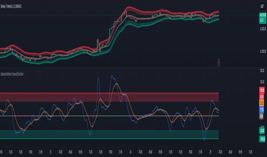
Advanced Keltner Channel/Oscillator [MyTradingCoder]This indicator combines a traditional Keltner Channel overlay with an oscillator, providing a comprehensive view of price action, trend, and momentum. The core of this indicator is its advanced ATR calculation, which uses statistical methods to provide a more robust measure of volatility.
Starting with the overlay component, the center line is created using a biquad low-pass filter applied to the chosen price source. This provides a smoother representation of price than a simple moving average. The upper and lower channel lines are then calculated using the statistically derived ATR, with an additional set of mid-lines between the center and outer lines. This creates a more nuanced view of price action within the channel.
The color coding of the center line provides an immediate visual cue of the current price momentum. As the price moves up relative to the ATR, the line shifts towards the bullish color, and vice versa for downward moves. This color gradient allows for quick assessment of the current market sentiment.
The oscillator component transforms the channel into a different perspective. It takes the price's position within the channel and maps it to either a normalized -100 to +100 scale or displays it in price units, depending on your settings. This oscillator essentially shows where the current price is in relation to the channel boundaries.
The oscillator includes two key lines: the main oscillator line and a signal line. The main line represents the current position within the channel, smoothed by an exponential moving average (EMA). The signal line is a further smoothed version of the oscillator line. The interaction between these two lines can provide trading signals, similar to how MACD is often used.
When the oscillator line crosses above the signal line, it might indicate bullish momentum, especially if this occurs in the lower half of the oscillator range. Conversely, the oscillator line crossing below the signal line could signal bearish momentum, particularly if it happens in the upper half of the range.
The oscillator's position relative to its own range is also informative. Values near the top of the range (close to 100 if normalized) suggest that price is near the upper Keltner Channel band, indicating potential overbought conditions. Values near the bottom of the range (close to -100 if normalized) suggest proximity to the lower band, potentially indicating oversold conditions.
One of the strengths of this indicator is how the overlay and oscillator work together. For example, if the price is touching the upper band on the overlay, you'd see the oscillator at or near its maximum value. This confluence of signals can provide stronger evidence of overbought conditions. Similarly, the oscillator hitting extremes can draw your attention to price action at the channel boundaries on the overlay.
The mid-lines on both the overlay and oscillator provide additional nuance. On the overlay, price action between the mid-line and outer line might suggest strong but not extreme momentum. On the oscillator, this would correspond to readings in the outer quartiles of the range.
The customizable visual settings allow you to adjust the indicator to your preferences. The glow effects and color coding can make it easier to quickly interpret the current market conditions at a glance.
Overlay Component:
The overlay displays Keltner Channel bands dynamically adapting to market conditions, providing clear visual cues for potential trend reversals, breakouts, and overbought/oversold zones.
The center line is a biquad low-pass filter applied to the chosen price source.
Upper and lower channel lines are calculated using a statistically derived ATR.
Includes mid-lines between the center and outer channel lines.
Color-coded based on price movement relative to the ATR.
Oscillator Component:
The oscillator component complements the overlay, highlighting momentum and potential turning points.
Normalized values make it easy to compare across different assets and timeframes.
Signal line crossovers generate potential buy/sell signals.
Advanced ATR Calculation:
Uses a unique method to compute ATR, incorporating concepts like root mean square (RMS) and z-score clamping.
Provides both an average and mode-based ATR value.
Customizable Visual Settings:
Adjustable colors for bullish and bearish moves, oscillator lines, and channel components.
Options for line width, transparency, and glow effects.
Ability to display overlay, oscillator, or both simultaneously.
Flexible Parameters:
Customizable inputs for channel width multiplier, ATR period, smoothing factors, and oscillator settings.
Adjustable Q factor for the biquad filter.
Key Advantages:
Advanced ATR Calculation: Utilizes a statistical method to generate ATR, ensuring greater responsiveness and accuracy in volatile markets.
Overlay and Oscillator: Provides a comprehensive view of price action, combining trend and momentum analysis.
Customizable: Adjust settings to fine-tune the indicator to your specific needs and trading style.
Visually Appealing: Clear and concise design for easy interpretation.
The ATR (Average True Range) in this indicator is derived using a sophisticated statistical method that differs from the traditional ATR calculation. It begins by calculating the True Range (TR) as the difference between the high and low of each bar. Instead of a simple moving average, it computes the Root Mean Square (RMS) of the TR over the specified period, giving more weight to larger price movements. The indicator then calculates a Z-score by dividing the TR by the RMS, which standardizes the TR relative to recent volatility. This Z-score is clamped to a maximum value (10 in this case) to prevent extreme outliers from skewing the results, and then rounded to a specified number of decimal places (2 in this script).
These rounded Z-scores are collected in an array, keeping track of how many times each value occurs. From this array, two key values are derived: the mode, which is the most frequently occurring Z-score, and the average, which is the weighted average of all Z-scores. These values are then scaled back to price units by multiplying by the RMS.
Now, let's examine how these values are used in the indicator. For the Keltner Channel lines, the mid lines (top and bottom) use the mode of the ATR, representing the most common volatility state. The max lines (top and bottom) use the average of the ATR, incorporating all volatility states, including less common but larger moves. By using the mode for the mid lines and the average for the max lines, the indicator provides a nuanced view of volatility. The mid lines represent the "typical" market state, while the max lines account for less frequent but significant price movements.
For the color coding of the center line, the mode of the ATR is used to normalize the price movement. The script calculates the difference between the current price and the price 'degree' bars ago (default is 2), and then divides this difference by the mode of the ATR. The resulting value is passed through an arctangent function and scaled to a 0-1 range. This scaled value is used to create a color gradient between the bearish and bullish colors.
Using the mode of the ATR for this color coding ensures that the color changes are based on the most typical volatility state of the market. This means that the color will change more quickly in low volatility environments and more slowly in high volatility environments, providing a consistent visual representation of price momentum relative to current market conditions.
Using a good IIR (Infinite Impulse Response) low-pass filter, such as the biquad filter implemented in this indicator, offers significant advantages over simpler moving averages like the EMA (Exponential Moving Average) or other basic moving averages.
At its core, an EMA is indeed a simple, single-pole IIR filter, but it has limitations in terms of its frequency response and phase delay characteristics. The biquad filter, on the other hand, is a two-pole, two-zero filter that provides superior control over the frequency response curve. This allows for a much sharper cutoff between the passband and stopband, meaning it can more effectively separate the signal (in this case, the underlying price trend) from the noise (short-term price fluctuations).
The improved frequency response of a well-designed biquad filter means it can achieve a better balance between smoothness and responsiveness. While an EMA might need a longer period to sufficiently smooth out price noise, potentially leading to more lag, a biquad filter can achieve similar or better smoothing with less lag. This is crucial in financial markets where timely information is vital for making trading decisions.
Moreover, the biquad filter allows for independent control of the cutoff frequency and the Q factor. The Q factor, in particular, is a powerful parameter that affects the filter's resonance at the cutoff frequency. By adjusting the Q factor, users can fine-tune the filter's behavior to suit different market conditions or trading styles. This level of control is simply not available with basic moving averages.
Another advantage of the biquad filter is its superior phase response. In the context of financial data, this translates to more consistent lag across different frequency components of the price action. This can lead to more reliable signals, especially when it comes to identifying trend changes or price reversals.
The computational efficiency of biquad filters is also worth noting. Despite their more complex mathematical foundation, biquad filters can be implemented very efficiently, often requiring only a few operations per sample. This makes them suitable for real-time applications and high-frequency trading scenarios.
Furthermore, the use of a more sophisticated filter like the biquad can help in reducing false signals. The improved noise rejection capabilities mean that minor price fluctuations are less likely to cause unnecessary crossovers or indicator movements, potentially leading to fewer false breakouts or reversal signals.
In the specific context of a Keltner Channel, using a biquad filter for the center line can provide a more stable and reliable basis for the entire indicator. It can help in better defining the overall trend, which is crucial since the Keltner Channel is often used for trend-following strategies. The smoother, yet more responsive center line can lead to more accurate channel boundaries, potentially improving the reliability of overbought/oversold signals and breakout indications.
In conclusion, this advanced Keltner Channel indicator represents a significant evolution in technical analysis tools, combining the power of traditional Keltner Channels with modern statistical methods and signal processing techniques. By integrating a sophisticated ATR calculation, a biquad low-pass filter, and a complementary oscillator component, this indicator offers traders a comprehensive and nuanced view of market dynamics.
The indicator's strength lies in its ability to adapt to varying market conditions, providing clear visual cues for trend identification, momentum assessment, and potential reversal points. The use of statistically derived ATR values for channel construction and the implementation of a biquad filter for the center line result in a more responsive and accurate representation of price action compared to traditional methods.
Furthermore, the dual nature of this indicator – functioning as both an overlay and an oscillator – allows traders to simultaneously analyze price trends and momentum from different perspectives. This multifaceted approach can lead to more informed decision-making and potentially more reliable trading signals.
The high degree of customization available in the indicator's settings enables traders to fine-tune its performance to suit their specific trading styles and market preferences. From adjustable visual elements to flexible parameter inputs, users can optimize the indicator for various trading scenarios and time frames.
Ultimately, while no indicator can predict market movements with certainty, this advanced Keltner Channel provides traders with a powerful tool for market analysis. By offering a more sophisticated approach to measuring volatility, trend, and momentum, it equips traders with valuable insights to navigate the complex world of financial markets. As with any trading tool, it should be used in conjunction with other forms of analysis and within a well-defined risk management framework to maximize its potential benefits.
SpectrumLibrary "Spectrum"
This library includes spectrum analysis tools such as the Fast Fourier Transform (FFT).
method toComplex(data, polar)
Creates an array of complex type objects from a float type array.
Namespace types: array
Parameters:
data (array) : The float type array of input data.
polar (bool) : Initialization coordinates; the default is false (cartesian).
Returns: The complex type array of converted data.
method sAdd(data, value, end, start, step)
Performs scalar addition of a given float type array and a simple float value.
Namespace types: array
Parameters:
data (array) : The float type array of input data.
value (float) : The simple float type value to be added.
end (int) : The last index of the input array (exclusive) on which the operation is performed.
start (int) : The first index of the input array (inclusive) on which the operation is performed; the default value is 0.
step (int) : The step by which the function iterates over the input data array between the specified boundaries; the default value is 1.
Returns: The modified input array.
method sMult(data, value, end, start, step)
Performs scalar multiplication of a given float type array and a simple float value.
Namespace types: array
Parameters:
data (array) : The float type array of input data.
value (float) : The simple float type value to be added.
end (int) : The last index of the input array (exclusive) on which the operation is performed.
start (int) : The first index of the input array (inclusive) on which the operation is performed; the default value is 0.
step (int) : The step by which the function iterates over the input data array between the specified boundaries; the default value is 1.
Returns: The modified input array.
method eMult(data, data02, end, start, step)
Performs elementwise multiplication of two given complex type arrays.
Namespace types: array
Parameters:
data (array type from RezzaHmt/Complex/1) : the first complex type array of input data.
data02 (array type from RezzaHmt/Complex/1) : The second complex type array of input data.
end (int) : The last index of the input arrays (exclusive) on which the operation is performed.
start (int) : The first index of the input arrays (inclusive) on which the operation is performed; the default value is 0.
step (int) : The step by which the function iterates over the input data array between the specified boundaries; the default value is 1.
Returns: The modified first input array.
method eCon(data, end, start, step)
Performs elementwise conjugation on a given complex type array.
Namespace types: array
Parameters:
data (array type from RezzaHmt/Complex/1) : The complex type array of input data.
end (int) : The last index of the input array (exclusive) on which the operation is performed.
start (int) : The first index of the input array (inclusive) on which the operation is performed; the default value is 0.
step (int) : The step by which the function iterates over the input data array between the specified boundaries; the default value is 1.
Returns: The modified input array.
method zeros(length)
Creates a complex type array of zeros.
Namespace types: series int, simple int, input int, const int
Parameters:
length (int) : The size of array to be created.
method bitReverse(data)
Rearranges a complex type array based on the bit-reverse permutations of its size after zero-padding.
Namespace types: array
Parameters:
data (array type from RezzaHmt/Complex/1) : The complex type array of input data.
Returns: The modified input array.
method R2FFT(data, inverse)
Calculates Fourier Transform of a time series using Cooley-Tukey Radix-2 Decimation in Time FFT algorithm, wikipedia.org
Namespace types: array
Parameters:
data (array type from RezzaHmt/Complex/1) : The complex type array of input data.
inverse (int) : Set to -1 for FFT and to 1 for iFFT.
Returns: The modified input array containing the FFT result.
method LBFFT(data, inverse)
Calculates Fourier Transform of a time series using Leo Bluestein's FFT algorithm, wikipedia.org This function is nearly 4 times slower than the R2FFT function in practice.
Namespace types: array
Parameters:
data (array type from RezzaHmt/Complex/1) : The complex type array of input data.
inverse (int) : Set to -1 for FFT and to 1 for iFFT.
Returns: The modified input array containing the FFT result.
method DFT(data, inverse)
This is the original DFT algorithm. It is not suggested to be used regularly.
Namespace types: array
Parameters:
data (array type from RezzaHmt/Complex/1) : The complex type array of input data.
inverse (int) : Set to -1 for DFT and to 1 for iDFT.
Returns: The complex type array of DFT result.

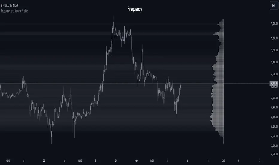
Frequency and Volume ProfileFREQUENCY & VOLUME PROFILE
⚪ OVERVIEW
The Frequency and Volume Profile indicator plots a frequency or volume profile based on the visible bars on the chart, providing insights into price levels with significant trading activity.
⚪ USAGE
● Market Structure Analysis:
Identify key price levels where significant trading activity occurred, which can act as support and resistance zones.
● Volume Analysis:
Use the volume mode to understand where the highest trading volumes have occurred, helping to confirm strong price levels.
● Trend Confirmation:
Analyze the distribution of trading activity to confirm or refute trends, mark important levels as support and resistance, aiding in making more informed trading decisions.
● Frequency Distribution:
In statistics, a frequency distribution is a list of the values that a variable takes in a sample. It is usually a list. Displayed as a histogram.
⚪ SETTINGS
Source: Select the price data to use for the profile calculation (default: hl2).
Move Profile: Set the number of bars to offset the profile from the current bar (default: 100).
Mode: Choose between "Frequency" and "Volume" for the profile calculation.
Profile Color: Customize the color of the profile lines.
Lookback Period: Uses 5000 bars for daily and higher timeframes, otherwise 10000 bars.
The Frequency Profile indicator is a powerful tool for visualizing price levels with significant trading activity, whether in terms of frequency or volume. Its dynamic calculation and customizable settings make it a versatile addition to any trading strategy.
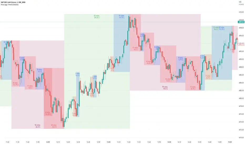
Price Legs: Time & Distance. Measuring moves in time & price-Tool to measure price legs in terms of both time and price; gives an idea of frequency of market movements and their typical extent and duration.
-Written for backtesting: seeing times of day where setups are most likely to unfold dynamically; getting an idea of typical and minimum sizes of small/large legs.
-Two sets of editable lookback numbers to measure both small and large legs independently.
-Works across timeframes and assets (units = mins/hours/days dependent on timeframe; units = '$' for indices & futures, 'pips' for FX).
~toggle on/off each set of bull/bear boxes.
~choose lookback/forward length for each set. Increase number for larger legs, decrease for smaller legs.
(for assets outside of the big Indices and FX, you may want to edit the multiplier, pMult, on lines 23-24)
small legs
large legs
FunctionPatternFrequencyLibrary "FunctionPatternFrequency"
Counts the word or integer number pattern frequency on a array.
reference:
rosettacode.org
count(pattern)
counts the number a pattern is repeated.
Parameters:
pattern : : array : array with patterns to be counted.
Returns:
array : list of unique patterns.
array : list of counters per pattern.
usage:
count(array.from('a','b','c','a','b','a'))
count(pattern)
counts the number a pattern is repeated.
Parameters:
pattern : : array : array with patterns to be counted.
Returns:
array : list of unique patterns.
array : list of counters per pattern.
usage:
count(array.from(1,2,3,1,2,1))

Fourier Extrapolator of Price w/ Projection Forecast [Loxx]Due to popular demand, I'm pusblishing Fourier Extrapolator of Price w/ Projection Forecast.. As stated in it's twin indicator, this one is also multi-harmonic (or multi-tone) trigonometric model of a price series xi, i=1..n, is given by:
xi = m + Sum( a*Cos(w*i) + b*Sin(w*i), h=1..H )
Where:
xi - past price at i-th bar, total n past prices;
m - bias;
a and b - scaling coefficients of harmonics;
w - frequency of a harmonic ;
h - harmonic number;
H - total number of fitted harmonics.
Fitting this model means finding m, a, b, and w that make the modeled values to be close to real values. Finding the harmonic frequencies w is the most difficult part of fitting a trigonometric model. In the case of a Fourier series, these frequencies are set at 2*pi*h/n. But, the Fourier series extrapolation means simply repeating the n past prices into the future.
This indicator uses the Quinn-Fernandes algorithm to find the harmonic frequencies. It fits harmonics of the trigonometric series one by one until the specified total number of harmonics H is reached. After fitting a new harmonic , the coded algorithm computes the residue between the updated model and the real values and fits a new harmonic to the residue.
see here: A Fast Efficient Technique for the Estimation of Frequency , B. G. Quinn and J. M. Fernandes, Biometrika, Vol. 78, No. 3 (Sep., 1991), pp . 489-497 (9 pages) Published By: Oxford University Press
The indicator has the following input parameters:
src - input source
npast - number of past bars, to which trigonometric series is fitted;
Nfut - number of predicted future bars;
nharm - total number of harmonics in model;
frqtol - tolerance of frequency calculations.
The indicator plots two curves: the green/red curve indicates modeled past values and the yellow/fuchsia curve indicates the modeled future values.
The purpose of this indicator is to showcase the Fourier Extrapolator method to be used in future indicators.

Fourier Extrapolator of Price [Loxx]Fourier Extrapolator of Price is a multi-harmonic (or multi-tone) trigonometric model of a price series xi, i=1..n, is given by:
xi = m + Sum( a *Cos(w *i) + b *Sin(w *i), h=1..H )
Where:
xi - past price at i-th bar, total n past prices;
m - bias;
a and b - scaling coefficients of harmonics;
w - frequency of a harmonic;
h - harmonic number;
H - total number of fitted harmonics.
Fitting this model means finding m, a , b , and w that make the modeled values to be close to real values. Finding the harmonic frequencies w is the most difficult part of fitting a trigonometric model. In the case of a Fourier series, these frequencies are set at 2*pi*h/n. But, the Fourier series extrapolation means simply repeating the n past prices into the future.
This indicator uses the Quinn-Fernandes algorithm to find the harmonic frequencies. It fits harmonics of the trigonometric series one by one until the specified total number of harmonics H is reached. After fitting a new harmonic, the coded algorithm computes the residue between the updated model and the real values and fits a new harmonic to the residue.
see here: A Fast Efficient Technique for the Estimation of Frequency , B. G. Quinn and J. M. Fernandes, Biometrika, Vol. 78, No. 3 (Sep., 1991), pp. 489-497 (9 pages) Published By: Oxford University Press
The indicator has the following input parameters:
src - input source
npast - number of past bars, to which trigonometric series is fitted;
nharm - total number of harmonics in model;
frqtol - tolerance of frequency calculations.
The indicator plots the modeled past values
The purpose of this indicator is to showcase the Fourier Extrapolator method to be used in future indicators. While this method can also prediction future price movements, for our purpose here we will avoid doing.

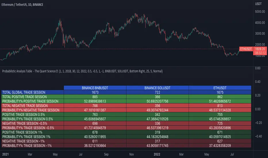
Probabilistic Analysis Table - The Quant ScienceProbabilistic Analysis Table - The Quant Science ™ is the quantitative table measuring the probability of price changes and quantifies the ratio of sessions for three different assets.
This table measures the ratios of bull and bear events and measures the probability of each event through data generated automatically by the algorithm.
The data are calculated for three different assets:
1. Main asset: set on the chart.
2. Second asset: set by user interface.
3. Third asset: set by the user interface.
The timeframe is set by the chart and is the same for all three assets. You can change the timeframes directly from the chart.
The user can add tickers and adjust the analysis period directly from the user interface. The user can edit the percentage changes and the values to be analyzed for each asset, directly from the user interface.
TABLE DESCRIPTION
1. Total global trade session: are the total number of bars for each asset.
2. Total positive trade session: are the number of positive bars for each asset.
3. Probability positive trade session: is the ratio of total sessions to positive sessions.
4. Total negative trade session: are the number of negative bars for each asset.
5. Probability negative trade session: is the ratio of total sessions to negative sessions.
6. Positive trade session 0.50%: are the number of positive bars greater than 0.50% for each asset.
7. Probability positive trade session 0.50%: is the ratio of total sessions to positive sessions with increases greater than 0.50% (this value is set by default, you can change it from the user interface).
8. Negative trade session -0.50%: are the number of negative bars smaller than -0.50% for each asset.
9. Probability negative trade session -0.50%: is the ratio of total sessions to negative sessions with declines less than -0.50% (this value is set by default, you can change it from the user interface).
10. Positive trade session 1%: are the number of positive bars greater than 1% for each asset.
11. Probability positive trade session 1%: is the ratio of total sessions to positive sessions with increases greater than 1% (this value is set by default, you can change it from the user interface).
12. Negative trade session -1%: are the number of negative bars less than -1% for each asset.
13. Probability negative trade session -1%: is the ratio of total sessions to negative sessions with declines less than -1% (this value is set by default, you can change it from the user interface).
This table was created for traders and quantitative investors who need to quickly analyze session ratios and probabilities.
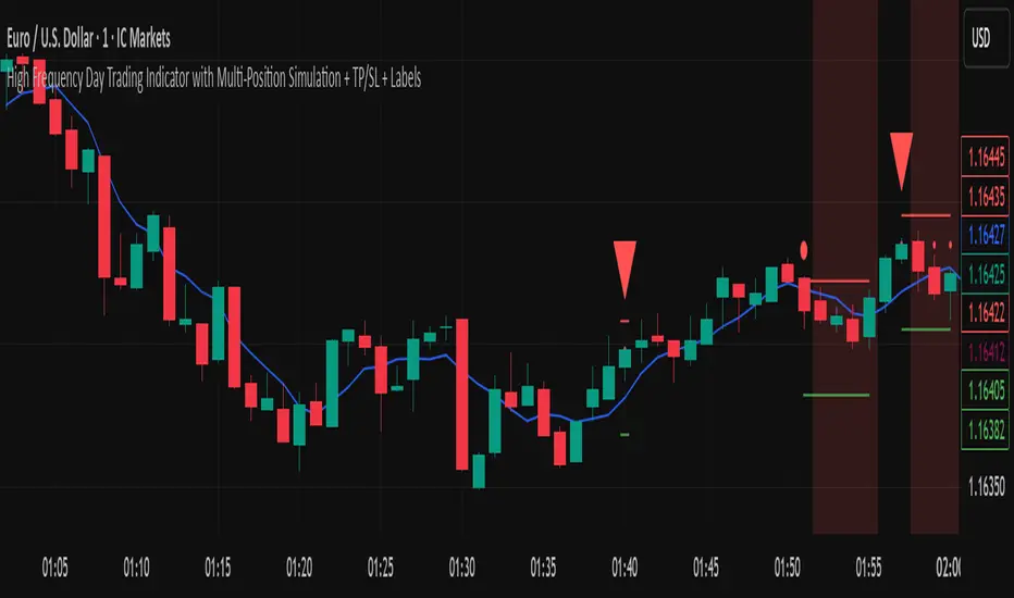
High Frequency Day Trading IndicatorMentioned Indicator uses RSI, Stoch RSI, SMA, EMA, SMMA, Double EMA to check for quick buying and selling areas for Day Trading.
For utilizing the tool, you'll need to wait for a Possible Trend Reversal (Represented by Triangle) and a confirmation to go Long by using a combination of Moving Averages which are then represented by circular dots on chart upon Bar Closure.
For Stop Loss once can simply place a Stop below/above the last Low/High respectively.
This trading Indicator is only recommended for high frequency trading on smaller time frames if you're using a highly volatile Coin/Asset Class.
Disclaimer: Please use this indicator in Test Environment to get a hold of concepts of this indicator. We do not advise using 100% capital for each order, as a matter of fact, we only recommend a risk of upto 1% on each position so Risk to Reward is maintained in proper sense. Please use Stops with all indicators and do not ever use an indicator without stop losses to save your capital.
NOTE: Indicator can be developed further to be used Trading Bots such as 3commas, Autoview, Wunderbit Bot, and Trailing Crypto Bots. For configuration of Automation Bots, you can contact us here on tradingview itself! :)
FunctionBestFitFrequencyLibrary "FunctionBestFitFrequency"
TODO: add library description here
array_moving_average(sample, length, ommit_initial, fillna) Moving Average values for selected data.
Parameters:
sample : float array, sample data values.
length : int, length to smooth the data.
ommit_initial : bool, default=true, ommit values at the start of the data under the length.
fillna : string, default='na', options='na', '0', 'avg'
Returns: float array
errors:
length > sample size "Canot call array methods when id of array is na."
best_fit_frequency(sample, start, end) Search a frequency range for the fairest moving average frequency.
Parameters:
sample : float array, sample data to based the moving averages.
start : int lowest frequency.
end : int highest frequency.
Returns: tuple with (int frequency, float percentage)

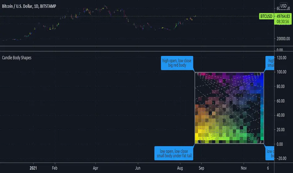
Candle Body ShapesExperimental:
displays the frequency of candle types.
reference: its a exploration of this topic: www.elitetrader.com
Tesla CoilThis indicator reads the charts as frequency because the charts are just waves after all. This is an excellent tool for finding "Booms" and detecting dumps. Booms are found when all the frequencies pull under the red 20 line. Dumps are detected when all the lines drag themselves along the 20 line as seen is screenshots below.
Below is another 2 examples of a "boom". Everything sucks in before exploding out.
Below is an example of a dump:

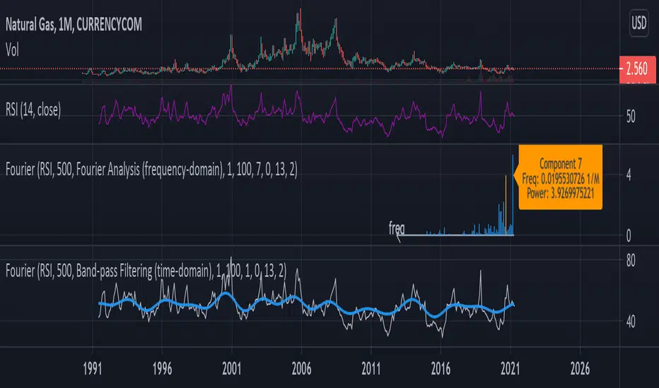
Fourier Analysis and Filtering [tbiktag]This tool uses Fourier transform to decompose the input time series into its periodic constituents and seasonalities , in other words, its frequency components . It also can reconstruct the time-domain data while using only the frequency components within a user-defined range (band-pass filtering). Thereby, this tool can reveal the cyclical characteristics of the studied market.
USAGE
The source and the size of the input data can be chosen by the “ Dataset Source ” and “ Dataset Size ” options. Price, volume, or some technical indicator (e.g., RSI, MACD, etc.) can serve as a source of the input data.
“ Action ” defines the type of the plot that will be displayed. Two options are available:
- Fourier Analysis
If selected, the frequency spectrum of the squares of the Fourier coefficient magnitudes is displayed. The zero-frequency component is on the right. Since the magnitudes of half of the coefficients are repeated, the graph displays only half of the frequency components.
The squared magnitude of a given frequency component is a measure of its power , that is, its contribution to the total variance of the dataset. Thus, by analyzing the frequency-domain spectrum, one can identify the most prominent seasonalities and then visualize them by using the " Band-pass Filtering " option (see below). Note that the zero component stores information about the amount of data, so it is naturally higher when the data is not centered at zero.
By activating the " Info about Frequency Component " option, the user can display information about the power and frequency of the selected Fourier component.
- Band-pass Filter
This option reconstructs and plots the dataset in the time domain, blocking frequency components outside of the cutoff frequencies (defined by the input parameters “ Upper Cutoff ” and “ Lower Cutoff ” input parameters in the “ Band-pass Filter Properties ” section).
FURTHER READING
In general, Fourier analysis has a long history of attempted applications for analyzing price data and estimating market cycles. For example, see the paper by John Ehlers
www.mesasoftware.com
and also some tools available here on TradingView, such as:
“Function: Discrete Fourier Transform” by @RicardoSantos
“Fourier series Model Of The Market” by @e2e4mfck
“Ehlers Discrete Fourier Transform” by @cheatcountry
Thus, I tried to make this tool versatile and user-friendly so you all can experiment with your own analysis.
Enjoy and don't hesitate to leave your feedback in the comments below!
Particle Physics Moving AverageThis indicator simulates the physics of a particle attracted by a distance-dependent force towards the evolving value of the series it's applied to.
Its parameters include:
The mass of the particle
The exponent of the force function f=d^x
A "medium damping factor" (viscosity of the universe)
Compression/extension damping factors (for simulating spring-damping functions)
This implementation also adds a second set of all of these parameters, and tracks 16 particles evenly interpolated between the two sets.
It's a kind of Swiss Army Knife of Moving Average-type functions; For instance, because the position and velocity of the particle include a "historical knowlege" of the series, it turns out that the Exponential Moving Average function simply "falls out" of the algorithm in certain configurations; instead of being configured by defining a period of samples over which to calculate an Exponential Moving Average, in this derivation, it is tuned by changing the mass and/or medium damping parameters.
But the algorithm can do much more than simply replicate an EMA... A particle acted on by a force that is a linear function of distance (force exponent=1) simulates the physics of a sprung-mass system, with a mass-dependent resonant frequency. By altering the particle mass and damping parameters, you can simulate something like an automobile suspension, letting your particle track a stock's price like a Cadillac or a Corvette (or both, including intermediates) depending on your setup. Particles will have a natural resonance with a frequency that depends on its mass... A higher mass particle (i.e. higher inertia) will resonate at a lower frequency than one with a lower mass (and of course, in this indicator, you can display particles that interpolate through a range of masses.)
The real beauty of this general-purpose algorithm is that the force function can be extended with other components, affecting the trajectory of the particle; For instance "volume" could be factored into the current distance-based force function, strengthening or weakening the impulse accordingly. (I'll probably provide updates to the script that incoroprate different ideas I come up with.)
As currently pictured above, the indicator is interpolating between a medium-damped EMA-like configuration (red) and a more extension-damped suspension-like configuration (blue).
This indicator is merely a tool that provides a space to explore such a simulation, to let you see how tweaking parameters affects the simulations. It doesn't provide buy or sell signals, although you might find that it could be adapted into an MACD-like signal generator... But you're on your own for that.

Filter Amplitude Response Estimator - A Simple CalculationIn digital signal processing knowing how a system interact with the frequency content of an input signal is extremely important, the mathematical tool that give you this information is called "frequency response". The frequency response regroup two elements, the amplitude response, and the phase response. The amplitude response tells you how the system modify the amplitude of the frequency components in the input signal, the phase response tells you how the system modify the phase of the frequency components in the signal, each being a function of the frequency.
The today proposed tool aim to give a low resolution representation of the amplitude response of any filter.
What Is The Amplitude Response Of A Filter ?
Remember that filters allow to interact with the frequency content of a signal by amplifying, attenuating and/or removing certain frequency components in the input signal, the amplitude (also called magnitude) response of a filter let you know exactly how your filter change the amplitude of the frequency components in the input signal, another way to see the amplitude response is as a tool that tell you what is the peak amplitude of a filter using a sinusoid of a certain frequency as input signal.
For example if the amplitude response of a filter give you a value of 0.9 at frequency 0.5, it means that the filter peak amplitude using a sinusoid of frequency 0.5 is equal to 0.9.
There are several ways to calculate the frequency response of a filter, when our filter is a FIR filter (the filter impulse response is finite), the frequency response of the filter is the absolute value of the discrete Fourier transform (DFT) of the filter impulse response.
If you are curious about this process, know that the DFT of a N samples signal return N values, so if our FIR filter coefficients are composed of only 5 values we would get a frequency response of 5 values...which would not be useful, this is why we "pad" our coefficients with zeros, that is we add zeros to the start and end of our series of coefficients, this process is called "zero-padding", so if our series of coefficients is: (1,2,3,4,5), applying zero padding would give (0,0...1,2,3,4,5,...0,0) while keeping a certain symmetry. This is related to the concept of resolution, a low resolution amplitude response would be composed of a low number of values and would not be useful, this is why we use zero-padding to add more values thus increasing the resolution.
Making a Fourier transform in Pinescript is not doable, as you need the complex number i for computing a DFT, but thats not even the only problem, a DFT would not be that useful anyway (as the processes to make it useful in a trading context would be way too complex) . So how can we calculate a filter amplitude response without using a DFT ? The simple answer is by taking the peak amplitude of a filter using a sinusoid of a certain frequency as input, this is what the proposed tool do.
Using The Tool
The proposed tool give you a 50 point amplitude response from frequency 0.005 to 0.25 by default. the setting "Range Divisor" allow you to see the amplitude response by using a different range of frequency, for example if the range divisor is equal to 2 the filter amplitude response will be evaluated from frequency 0.0025 to 0.125.
In the script, filt hold the filter you want to see the frequency response, by default a simple moving average.
The position of the frequency response is defined by the "Show Amplitude Response At Bar Number" setting, if you want the frequency response to start at bar number 5000 then enter 5000, by default 10000. If you are not a premium set the number at 4000 and it should work.
amplitude response of a simple moving average of period 14, res = 2.
By default the amplitude response use an amplitude scale, a value of 1 represent an unchanged amplitude. You can use Dbfs (decibel full scale) instead by checking the "To Decibels (Full Scale)" setting.
Dbfs amplitude response, a value of 0 represent an unchanged amplitude.
Some Amplitude Responses
In order to prove the accuracy of the proposed tool we can compare the amplitude response given by the proposed tool with the mathematical function of the amplitude response of a simple moving average, that is:
abs(sin(pi*f*length)/(length*sin(pi*f)))
In cyan the amplitude response given by the proposed tool and in blue the above function. Below are the amplitude responses of some moving averages with period 14.
Amplitude response of an EMA, the EMA is a IIR filter, therefore the amplitude response can't be made by taking the DFT of the impulse response (as this ones has infinite length), however our tool can give its frequency response.
Amplitude response of the Hull MA, as you can see some frequencies are amplified, this is common with low-lag filters.
Gaussian moving average (ALMA), with offset = 0.5 and sigma = 6.
Simple moving average high-pass filter amplitude response
Center of gravity bandpass filter amplitude response
Center of gravity bandreject filter.
IMPORTANT!: The amplitude response of adaptive moving averages is not stationary and might change over time.
Conclusion
A tool giving the amplitude response of any filter has been presented, of course this method is not efficient at all and has a low resolution of 50 points (the common resolution is of 512 points) and is difficult to work with, but has the merit to work on Tradingview and can give the frequency response of IIR filters, if you really need to see the frequency response of a filter then i recommend you to use the function freqz from the scipy package.
I still hope you will enjoy using this tool to have a look at the amplitude responses of your favorite moving averages.
I'am aware of the current situation, however i'am somehow feeling left out from the pinescript community, let me know via PM if i have done something to you and i'll do my best to fix any problems i might have caused (or i might be being parano xD)
