Key Levels: Volume Profile POCProfessional Intraday Key Levels (CST)
This is a comprehensive, institutional-grade Pine Script indicator designed for intraday traders (Futures, Stocks, Options) operating in the Central Time Zone. It automatically plots the most significant support and resistance levels used by algorithms and professional desks.
1. Core Levels Monitored
Daily Levels: Previous Day High (PDH), Low (PDL), Open, Close, and the 50% Midpoint (Equilibrium).
Volume Profile POC: Unlike standard indicators that use a simple average, this calculates the Volume Weighted Average Price (VWAP) of the previous day to determine the true "Fair Value" or Point of Control. Plotted with a thicker, distinct purple line.
Weekly Magnets: Previous Week High (PWH) and Low (PWL), which often act as major targets for breakouts or reversals.
Pre-Market Data: Tracks the High and Low established between 03:00 AM – 08:30 AM CST.
Opening Range (OR): Automatically captures the High and Low of the first 60 minutes of the regular session (08:30 AM – 09:30 AM CST).
2. Smart Visualization Features
Anti-Overlap Labels: If two levels (e.g., Pre-Market High and Previous Day High) are within 0.02% of each other, the script automatically merges them into a single label (e.g., "PDH & Pre-Market High") to prevent chart clutter.
Source Tracing: Trace lines extend backward from the current price level to the exact candle where that High or Low was formed (for Pre-Market and Opening Range levels), giving you instant context on when the level was created.
Clean Readability: Labels are displayed in bold, solid text without price numbers, ensuring a clean chart that focuses on level identification rather than data overload.
3. Technical Precision
Time Zone Locked: Hardcoded to America/Chicago to ensure Pre-Market and Opening Range calculations remain accurate regardless of your local computer settings.
Non-Repainting: Daily and Weekly levels are locked using closed-candle data (lookahead_on), ensuring lines do not shift during the trading day.
Buffer Safe: Optimized drawing logic prevents historical buffer errors, even on lower timeframes (1m/5m).
4. Customization
Toggle Everything: Every single level has an individual "Show/Hide" checkbox in the settings.
Label Sizing: Adjustable text size (Tiny to Huge) and offset positioning.
Compact Mode: Option to switch between full names ("Previous Day High") and abbreviations ("PDH").
사이클

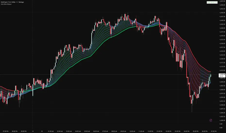
Danny Gee EMA Trend RibbonDanny Gee EMA Trend Ribbon - Multi-Timeframe Trend Analysis
A sophisticated 9-EMA ribbon system designed to visualize trend strength and direction with precision. This indicator creates a dynamic color-coded ribbon that adapts to market conditions, making trend identification effortless.
Key Features:
9 Customizable EMAs - Default periods: 8, 14, 20, 26, 32, 38, 44, 50, and 60
Intelligent Ribbon Coloring - Automatically displays bullish (green), bearish (red), or neutral (gray) based on EMA consensus
Smoothing Control - Adjustable smoothing period (default 2) reduces noise and false signals
Real-Time Trend Status - Live dashboard showing current trend state and EMA agreement count (e.g., "Bullish 8/9")
Visual Clarity - Color-coded EMA lines with the 60 EMA highlighted for key support/resistance
How It Works:
The indicator analyzes the slope direction of all 9 EMAs. When 7 or more EMAs agree on direction, the ribbon displays a clear bullish or bearish color. This consensus-based approach helps filter out weak or conflicting trends, keeping you focused on high-probability setups.
Best Used For:
✓ Identifying strong trending conditions
✓ Avoiding choppy, sideways markets
✓ Confirming trade direction with other indicators
✓ Multi-timeframe analysis (works on any chart timeframe)
Customization Options:
Adjust all EMA periods to match your trading style
Customize ribbon colors for personal preference
Toggle ribbon visibility on/off
Modify smoothing sensitivity
Perfect for swing traders, scalpers, and day traders looking for a clean, reliable trend filter that works across all markets - forex, crypto, stocks, and indices.
My RSI Fib Range Cloud//SOLO900q99This is basically the close price, optionally “stepped” if you set Bars Per Sample > 1.
2. Central Threshold Band (colored line)
• This is an EMA of the resampled price (default length 34).
• It turns:
• Green when RSI is in bullish fib zones,
• Pink when RSI is in bearish fib zones,
• Grey when RSI is in the middle/neutral area.
3. Sigma Range High (green line) and Sigma Range Low (pink line)
• These are an upper and lower band around price.
• The distance from price is based on how much price has been moving recently (average change).

Dipy the MFT Super OscillatorDipy the MFT Super Oscillator
A multi-timeframe bandpass oscillator for mean-reversion and "buy the dip" strategies.
🎯 What It Does
Isolates market cycles within a specific frequency range to identify overbought/oversold conditions and reversal points.
⏱️ Multi-Timeframe
Set Signal Timeframe to calculate signals on higher TF while viewing lower TF chart. Example: 5min chart + 1H signals = noise reduction with precise timing.
⚙️ Key Settings
Bandwidth/BandEdge: Define the cycle range to capture
Cloud Type: None for thresholds, others for consensus cloud
Thresholds: Overbought/oversold levels for signals
💡 Best Use
Combine with trend indicator (only buy dips in uptrend)
Higher Signal Timeframe = cleaner signals
Cloud mode = more conservative entries
🔔 Alerts
Create ONE alert for all signals.
Derived from TASC 2025.04 Ultimate Oscillator by John Ehlers.


Box Theory StrategyHere is an explanation of the Box Theory trading strategy.
The Core Philosophy
This strategy is based on the idea that the market is a battle between buyers and sellers, and that these groups often defend the same price levels they used previously. Instead of trying to predict every move, this method focuses on trading only at the "extremes" where the probabilities are highest, while avoiding the middle of the chart where price action is random.
1. The Setup: Drawing the Box
To use this strategy, you must define the "playing field" for the day before you take any trades.
Top of the Box: Draw a line at the Previous Day’s High.
Bottom of the Box: Draw a line at the Previous Day’s Low.
Center Line: Draw a line roughly in the middle of these two points.
This box represents the established range where the market recently found value.
2. The Three Zones & Rules
Once the box is drawn, the chart is divided into three zones. Each zone dictates a specific action.
Zone 1: The Top (Resistance / Sell Zone)
What it represents: This is where sellers previously stepped in and pushed the price down. It is a known area of supply.
The Rule: NO BUYING.
If the price rallies to this level, you should look for Short/Sell opportunities.
Why? Buying here means purchasing at a price that was previously rejected. The probability of a reversal (price going down) is high.
Zone 2: The Bottom (Support / Buy Zone)
What it represents: This is where buyers previously stepped in and pushed the price up. It is a known area of demand.
The Rule: NO SELLING.
If the price drops to this level, you should look for Long/Buy opportunities.
Why? Selling here means shorting into support. The probability of a bounce (price going up) is high.
Zone 3: The Middle (Indecision Zone)
What it represents: This is the area of noise and confusion. Neither buyers nor sellers have clear control here.
The Rule: DO NOT TRADE.
Why? In the middle of the range, the odds of the price going up or down are roughly 50/50. Trading here is considered gambling because you do not have a statistical edge.
3. Execution: How to Trade
The Entry
Short Setup: Wait for the price to touch or slightly pierce the Top of the Box. Enter a short position when you see the price failing to break out (e.g., leaving a wick and closing back inside the box).
Long Setup: Wait for the price to touch or slightly pierce the Bottom of the Box. Enter a long position when you see the price failing to break down (e.g., bouncing off the level).
Stop Loss (Risk Management)
This strategy offers a very clear invalidation point.
For Shorts: Place your Stop Loss just above the box.
For Longs: Place your Stop Loss just below the box.
Logic: If the price clearly breaks out of the box, the range is broken, and you want to exit the trade immediately with a small loss.
Take Profit (Targets)
First Target: The Center Line. This is a safe place to take some profit or move your stop loss to breakeven.
Main Target: The opposite side of the box (e.g., if you sold at the top, target the bottom).
4. Handling Gaps (The "Cheater Box")
If the market opens significantly higher or lower than the previous day's range (a large gap), the original box may be too far away to be useful.
Adjustment: In this scenario, you can draw a new box using the highest and lowest price points of the current trading session so far.
Once this new range is established, apply the same rules: Sell the high, Buy the low, and avoid the middle.

GARCH Adaptive Volatility & Momentum Predictor
💡 I. Indicator Concept: GARCH Adaptive Volatility & Momentum Predictor
-----------------------------------------------------------------------------
The GARCH Adaptive Momentum Speed indicator provides a powerful, forward-looking
view on market risk and momentum. Unlike standard moving averages or static
volatility indicators (like ATR), GARCH forecasts the Conditional Volatility (σ_t)
for the next bar, based on the principle of volatility clustering.
The indicator consists of two essential components:
1. GARCH Volatility (Level): The primary forecast of the expected magnitude of
price movement (risk).
2. Vol. Speed (Momentum): The first derivative of the GARCH forecast, showing
whether market risk is accelerating or decelerating. This component is the
main visual signal, displayed as a dynamic histogram.
⚙️ II. Key Features and Adaptive Logic
-----------------------------------------------------------------------------
* Dynamic Coefficient Adaptation: The indicator automatically adjusts the GARCH
coefficients (α and β) based on the chart's timeframe (TF):
- Intraday TFs (M1-H4): Uses higher α and lower β for quicker reaction
to recent shocks.
- Daily/Weekly TFs (D, W): Uses lower α and higher β for a smoother,
more persistent long-term forecast.
* Momentum Visualization: The Vol. Speed component is plotted as a dynamic
histogram (fill) that automatically changes color based on the direction of
acceleration (Green for up, Red for down).
📊 III. Interpretation Guide
-----------------------------------------------------------------------------
- GARCH Volatility (Blue Line): The predicted level of market risk. Use this to
gauge overall position sizing and stop loss width.
- Vol. Speed (Green Histogram): Momentum is ACCELERATING (Risk is increasing rapidly).
A strong signal that momentum is building, often preceding a breakout.
- Vol. Speed (Red Histogram): Momentum is DECELERATING (Risk is contracting).
Indicates momentum is fading, often associated with market consolidation.
🎯 IV. Trading Application
-----------------------------------------------------------------------------
- Breakout Timing: Look for a strong, high GREEN histogram bar. This suggests
the volatility pressure is increasing rapidly, and a breakout may be imminent.
- Consolidation: Small, shrinking RED histogram bars signal that market energy
is draining, ideal for tight consolidation patterns.

Daily & Pre-Market Key Levels (v5)Plots:
- Today's high/low
- Pre-market High/Low
- Yesterday's high/low/close
- Day before yesterday high/low

TASC 2026.01 The Reversion Index█ OVERVIEW
This script implements the Reversion Index as presented by John F. Ehlers in the January 2026 edition of the TASC Traders' Tips , "Identifying Peaks And Valleys In Ranging Markets”. This indicator was created to provide timely buy and sell signals for mean reversion strategies.
█ CONCEPTS
Ehlers came up with the idea for the Reversion Index following the development of the "Continuation Index" (featured in the September 2025 edition). While the Continuation Index provides indications for trend onset, continuation, and exhaustion; the Reversion Index serves as its counterpart for mean-reversion trading.
The raw Reversion Index value is calculated as the net change in price normalized to the sum of the absolute value of change in price over the same period; for clarity, it is then smoothed using Ehlers' SuperSmoother.
The Smooth Reversion Index value is led by a "Trigger" line, which is created by smoothing the raw data to half the smoothing period of the smoothed index.
Note: Ehlers suggests the smoothing lengths be left at 8 and 4 (Reversion Index & Trigger). For this reason these lengths are hard-coded in the script but can be easily modified in the code.
█ USAGE
In order to identify peaks and valleys effectively, the "Length" should ideally be set to half of that of the expected cycle of the data. If the expected cycle of your trading data is 20 bars, a 10 bar length should be set.
Note: The Reversion Index is intended to identify peaks and valleys within a cycle, not over a large sample period. Ehlers suggests that this would create an estimation of trend, which is not the goal here.
Once the length is set, peaks and valleys are interpreted as the cross of the "Trigger" and "Smooth" lines.

Selected Days Indicator V3-TrDoes the stock drop every Wednesday? Do March months always move similarly? Does the 1st week of the month behave differently?
Do you ever say "it always makes this move in these months"? Don't you want to see more clearly whether it actually makes this move or not? Don't you want to see and test periodically repeating price patterns?
Hisse her Çarşamba düşüyor mu? Mart ayları hep benzer mi hareket ediyor? Ayın 1. haftası farklı mı davranıyor?
Bazen "bu aylarda hep bu hareketi yapıyor" dediğiniz oluyor mu? Gerçekten de bu hareketi yapıp yapmadığını daha net görmek istemez misiniz? Periyodik tekrarlayan fiyat kalıplarını görmek ve test etmek istemiyor musunuz?
1. Problem
Some stocks or crypto assets exhibit systematic behaviors on certain days, weeks, or months. But it's hard to see - everything is mixed together on the chart. This indicator isolates the days/weeks/months you want and shows only them. Hides everything else.
2. How It Works
Three-layer filter: Day (Monday, Tuesday...), Week (1st, 2nd, 3rd week of the month), Month (January, February...). Select what you want, let the rest disappear. Example: Show only Thursdays of March-June-September. Or compare every 1st week of the month. View as candlestick, line, or column chart.
3. What's It Good For?
Test "end-of-month effect". Find "day-of-the-week anomaly". Analyze crypto volatility by days. See seasonality in commodities. Discover patterns specific to your own strategy. Past data doesn't guarantee the future but provides statistical advantage.

Pivot Points High LowGaneshA Pivot Points High/Low indicator that:
Detects swing highs (ta.pivothigh) and swing lows (ta.pivotlow) using configurable left/right bar lengths.
Draws labels at the confirmed pivot points:
Down labels at pivot highs (potential resistance).
Up labels at pivot lows (potential support).
Lets you customize text color and label fill color separately for highs and lows.
It’s designed for overlay (on-price chart), with max_labels_count=500 to allow many labels.
Highlighted Range (3 Sessions)3 session customizable range. All one color customizable for simplicity.

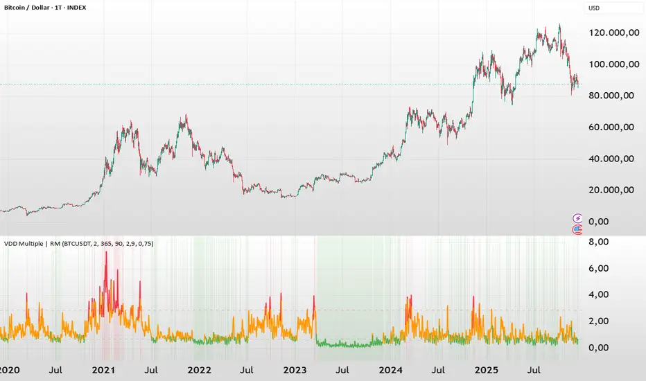
BTC - VDD Multiple (Approx)Overview & Philosophy
⚠️ Note: This indicator is optimized for the Daily (1D) Timeframe. Please switch your chart to 1D for accurate signal reading.
The BTC – VDD Multiple (Approx) is an advanced oscillator designed to identify market overheating and cycle tops by analyzing the velocity of value moving through the market.
In traditional On-Chain Analysis, Value Days Destroyed (VDD) is a premier metric for spotting macro tops. It multiplies the coin age (how long a coin was held) by the price at which it was moved. When old coins (HODLer money) move at high prices, VDD spikes, signaling massive profit-taking.
The Problem: Real "Coin Days Destroyed" (CDD) data is typically locked behind institutional paywalls or unavailable on standard TradingView plans.
The Solution: This script calculates a Deterministic Proxy. By analyzing the relationship between Exchange Volume, Price, and a Dormancy Constant, we can approximate the structure of the VDD Multiple without needing a premium data feed.
Methodology
The VDD Multiple works by comparing short-term market velocity against a long-term baseline.
1. The Proxy Calculation
Since we cannot directly access the age of coins on TradingView, we model the economic weight of the move:
Proxy Value = Exchange Volume * Price * Dormancy Factor
This creates a synthetic representation of "Value Throughput."
2. The Multiple
We compare the immediate heat of the market against the yearly trend:
• Short-Term MA (2 Days): Captures flash spikes and sudden liquidity exit events.
• Long-Term MA (365 Days): Represents the baseline "hum" of network activity.
VDD Multiple = Short Term MA / Long Term MA
How to Read the Chart
The indicator plots the Multiple as a line and uses background highlighting to signal extreme regimes.
🔴 The Red Zone (Overheated > 2.9)
Meaning: Current value transfer is ~3x higher than the yearly average.
Interpretation: Historically, sharp spikes into the Red Zone correlate with Local or Cycle Tops. This indicates that massive volume is changing hands at high prices—typically a sign of "Smart Money" distributing into "Dumb Money" FOMO.
Note: In strong bull runs, price can push higher even after a VDD spike, but the risk/reward ratio is extremely poor here.
🟢 The Green Zone (Undervalued < 0.75)
Meaning: Market activity is quiet and below the yearly baseline.
Interpretation: These are periods of apathy or accumulation. Historically, extended time spent in the Green Zone (the "flatline") has offered the best asymmetric buying opportunities.
🟠 The Orange Line (Neutral)
Meaning: The market is in transition or equilibrium.
Strategy & Context
This indicator is best used as a Macro Cycle Tool, not a day-trading signal.
• Exit Strategy: Look for "Clusters" of Red Spikes. A single spike often marks a local correction, but a cluster of intense spikes while price makes new highs (Divergence) is a strong Cycle Top warning.
• Entry Strategy: Historically the best entries occur when the indicator flattens out in the Green Zone for weeks or months. This suggests sellers are exhausted and the market has reached a floor.
Credits
This script is an approximation of the original VDD Multiple concept. Full credit for the underlying on-chain theory goes to the pioneers of this metric:
• Concept: The original Value Days Destroyed metric was popularized by Hans Hauge and Glassnode.
• The Multiple: The specific application of a Short/Long MA Multiple on VDD is widely attributed to analysts like TXMC and Bitbo.
This script adapts these concepts for the free TradingView environment using exchange volume proxies.
Settings
• Data Source: Defaults to BINANCE:BTCUSDT to capture high-volume liquidity.
• Short MA: Default is 2 Days to capture rapid velocity spikes.
• Long MA: Default is 365 Days to track the annual trend.
Disclaimer
This tool is an approximation based on exchange volume, not raw blockchain data. While exchange volume and on-chain volume are highly correlated during cycle extremes, they are not identical. This script is for educational and research purposes only. Past performance does not guarantee future results.
Tags
bitcoin, btc, onchain, vdd, cdd, valuation, cycle, top, bottom, Rob Maths
Multi-Trend + Credit Risk DashboardHello This is showing 20,50,200 as well as some other useful indicators. hope you like it, its my first! D and P is discount or premium to nav

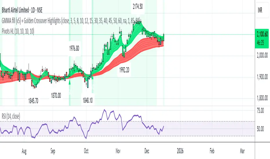
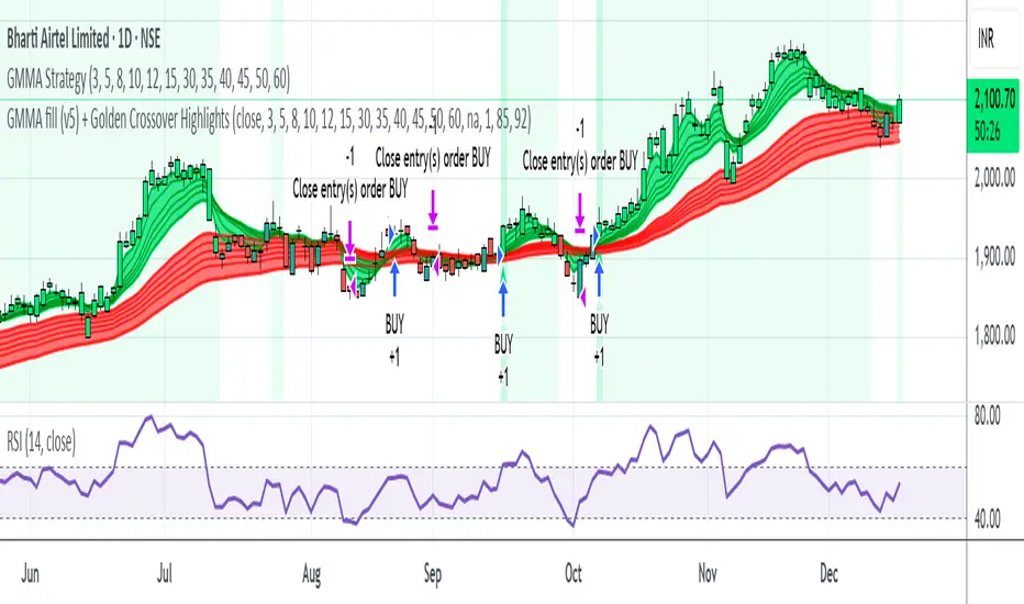
GMMA fill (v5) + Golden Crossover HighlightsGMMA Fill (v5) + Golden Crossover Highlights
This setup combines the Guppy Multiple Moving Average (GMMA) Fill version 5 with Golden Crossover signals to identify strong trend continuation and potential breakout points. GMMA provides layered moving averages for short- and long-term trend analysis, while the Golden Crossover highlights bullish momentum shifts, making it ideal for spotting entry opportunities in trending markets.
Rainbow MA Cloud█ OVERVIEW
Rainbow MA Cloud displays 8 Moving Averages as a gradient-colored cloud to visualize trend direction and strength. The "rainbow" effect shows momentum through ribbon width, while perfect MA alignment signals strong trending conditions.
█ CONCEPTS
The indicator uses 8 MAs with Fibonacci-based default lengths (8, 13, 21, 34, 55, 89, 144, 233) to create a layered view of price momentum across multiple timeframes.
Perfect Alignment Detection:
• Bullish Alignment — All 8 MAs in ascending order (MA1 > MA2 > ... > MA8)
Indicates strong uptrend with momentum across all timeframes
• Bearish Alignment — All 8 MAs in descending order (MA1 < MA2 < ... < MA8)
Indicates strong downtrend with aligned selling pressure
• Mixed — MAs are not in sequential order, suggesting consolidation or transition
Ribbon Width:
• Widening ribbon = Trend acceleration, increasing momentum
• Narrowing ribbon = Trend weakening, potential reversal or consolidation
█ FEATURES
1 — MA Configuration
Choose from EMA, SMA, WMA, VWMA, or HMA calculation methods.
All 8 MA lengths are fully customizable.
2 — Color Themes
Five built-in themes: Rainbow, Warm, Cool, Neon, Mono.
Creates visually distinct gradient from fast to slow MAs.
3 — Alignment Background
Green background during bullish alignment.
Red background during bearish alignment.
Helps quickly identify strong trending periods.
4 — Trend Signals
Labels appear when perfect alignment forms.
"BULL ALIGN" for bullish, "BEAR ALIGN" for bearish.
5 — Information Panel
Real-time display of alignment status, trend strength percentage,
ribbon width, price position relative to cloud, and MA values.
█ HOW TO USE
Entry Signals:
• Look for alignment signals (BULL/BEAR ALIGN) as trend confirmation
• Enter long when bullish alignment forms with price above cloud
• Enter short when bearish alignment forms with price below cloud
Trend Following:
• Stay in position while alignment background color persists
• Widening ribbon confirms trend continuation
• Exit or reduce when alignment breaks (background disappears)
Support/Resistance:
• Cloud edges act as dynamic support (bullish) or resistance (bearish)
• Price entering cloud suggests consolidation or potential reversal
█ LIMITATIONS
• Alignment signals are lagging by nature (based on MA crossovers)
• Works best on trending markets; generates mixed signals during ranging periods
• Ribbon width measurement uses outer MAs only (MA1 vs MA8)
█ COMPANION INDICATOR
Use "Rainbow MA Width" indicator for detailed Z-Score analysis of ribbon expansion/contraction patterns.

BTC - ALSI: Altcoin Season Index (Dynamic Eras)Title: BTC - ALSI: Altcoin Season Index (Dynamic Eras)
Overview & Philosophy
The Altcoin Season Index (ALSI) is a quantitative tool designed to answer the most critical question in crypto capital rotation: "Is it time to hold Bitcoin, or is it time to take risks on Altcoins?"
Most "Altseason" indicators suffer from Survivor Bias or Obsolescence. They either track a static list of coins that includes "dead" assets from previous cycles (ghosts of 2017), or they break completely when major tokens collapse (like LUNA or FTT).
This indicator solves this by using a Time-Varying Basket. The indicator automatically adjusts its reference list of Top 20 coins based on historical eras. This ensures the index tracks the winners of the moment—capturing the DeFi summer of 2020, the NFT craze of 2021, and the AI/Meme narratives of 2024/2025.
Methodology
The indicator calculates the percentage of the Top 20 Altcoins that are outperforming Bitcoin over a rolling window (Default: 90 Days).
The "Win" Count: For every major Altcoin performing better than BTC, the index adds a point.
Dynamic Eras: The basket of coins changes depending on the date:
2020 Era (DeFi Summer): Tracks the "Blue Chips" of the DeFi revolution like UNI, LINK, DOT, and early movers like VET and FIL.
2021 Era (Layer 1 Wars): Tracks the explosion of alternative smart contract platforms, adding winners like SOL, AVAX, MATIC, and ALGO.
2022 Era (The Survivors): Filters for resilience during the Bear Market, solidifying the status of established assets like SHIB and ATOM.
2023 Era (Infrastructure & Scale): Captures the rise of "Next-Gen" tech leading into the pre-halving year, introducing TON, APT (Aptos), and ARB (Arbitrum).
2024/25 Era (AI & Speed): Tracks the current Super-Cycle leaders, focusing on the AI narrative (TAO, RNDR), High-Performance L1s (SUI), and modern Memes (PEPE).
Chart Analysis & Strategy ( The "Alpha" )
As seen in the chart above, there is a strong correlation between ALSI Peaks and local tops in TOTAL3 (The Crypto Market Cap excluding BTC & ETH).
The Entry (Rotation): When the indicator rises above the neutral 50 line, it signals that capital is beginning to rotate out of Bitcoin and into Altcoins. This has historically been a strong confirmation signal to increase exposure to high-beta assets.
The Exit (Saturation): When the indicator hits 100 (or sustains in the Red Zone > 75), it means every single Altcoin is beating Bitcoin. Historically, this extreme exuberance often marks a local top in the TOTAL3 chart. This is the zone where smart money typically sells into strength, rather than opening new positions.
How to Read the Visuals
🚀 Altcoin Season (Red Zone > 75): Strong Altcoin dominance. The market is "Risk On."
🛡️ Bitcoin Season (Blue Zone < 25): Bitcoin dominance. Alts are bleeding against BTC. Historically, this is a defensive zone to hold BTC or Stablecoins.
Data Dashboard: A status table in the bottom-right corner displays the live Index Value, current Regime, and a System Check to ensure all 20 data feeds are active.
Settings
Lookback Period: Default 90 Days. Lowering this (e.g., to 30) makes the index faster but noisier.
Thresholds: Adjustable zones for Altcoin Season (Default: 75) and Bitcoin Season (Default: 25).
Credits & Attribution
This open-source indicator is built on the shoulders of giants. I acknowledge the original creators of the concept and the pioneers of its implementation on TradingView:
Original Concept: BlockchainCenter.net. - They established the industry standard definition: 75% of the Top 50 coins outperforming Bitcoin over 90 days = Altseason..
TradingView Implementation: Adam_Nguyen - He implemented the "Dynamic Era" logic (updating the coin list annually) on TradingView. Our code structure for the time-based switching is inspired by his methodology. See also his implementation in the chart. ( Altcoin Season Index - Adam) .
Comparison: Why use ALSI | RM?
While inspired by the above, ALSI introduces three key improvements:
Open Source: Unlike other popular TradingView versions (which are closed-source), this script is fully transparent. You can see exactly which coins are triggering the signal.
Sanitized History (Anti-Fragile): Historical Top 20 snapshots are not blindly used. "Dead" coins (like LUNA and FTT) from previous eras are manually filtered out. A raw index would crash during the Terra/FTX collapses, giving a false "Bitcoin Season" signal purely due to bad actors. The curated list preserves the integrity of the market structure signal.
Narrative Relevance: The 2024/25 basket was updated to include TAO (Bittensor) and RNDR, ensuring the index captures the dominant AI narrative, rather than tracking fading assets from the previous cycle.
You can compare the ALSI indicator with other available tradingview indicators in the chart: Different indicators for the same idea are shown in the 3 Pane window below the BTC and Total3 chart, whereas ALSI is the top pane indicator.
Important Note on Coin Selection Baskets are highly curated: Dead/irrelevant coins (FTT, LUNA, BSV) are excluded for clean signals. This prevents historical breaks and ensures Era T5 captures current narratives (AI, Memes) via TAO/RNDR. See above. Users are free to adjust the source code to test their own baskets.
Disclaimer
This script is for research and educational purposes only. Past correlations between ALSI and TOTAL3 do not guarantee future results. Market regimes can change, and "Altseasons" can be cut short by macro events.
Tags
bitcoin, btc, altseason, dominance, total3, rotation, cycle, index, alsi, Rob Maths

Fish vs Shark Vote Dashboard (6 Signals)very simple dashboard align with fish and shark market votes 1/5 2/4 etc

Day of WeekDay of Week is an indicator that runs in a separate panel and colors the panel background according to the day of the week.
Main Features
Colors the background of the lower panel based on the day of the week
Includes all days, from Monday to Sunday
Customizable colors
Time Offset Correction
TradingView calculates the day of the week using the exchange’s timezone, which can cause visual inconsistencies on certain symbols.
To address this, the indicator includes a configurable time offset that allows the user to synchronize the calculated day with the day displayed on the chart.
By simply adjusting the Time Offset (hours) parameter, the background will align correctly with the visible chart calendar.

Monthly Hotness RSI (Auto-Calibrated)Indicator of the previous months volatility/vol compared to averages over the last 3-5 years. helps show trend and if the market is 'hot'. indicator is good for showing favourable market conditions.

DZDZ – Pivot Demand Zones + Trend Filter + Breadth Override + SL is a structured accumulation indicator built to identify high-probability demand areas after valid pullbacks.
The script creates **Demand Zones (DZ)** by pairing **pivot troughs (local lows)** with later **pivot peaks (local highs)**, requiring a minimum **ATR (Average True Range)** gap to confirm real price displacement. Zones are drawn only when market structure confirms strength through a **trend filter** (a required number of higher highs over a recent window) or a **breadth override**, which activates after unusually large expansion candles measured as a percentage move from the prior close.
In addition to pivots, the script detects **coiling price action**—tight trading ranges contained within an ATR band—and treats these as alternative demand bases.
Entries require price to penetrate a defined depth into the zone, preventing shallow reactions. After the first valid entry, a **DCA (Dollar-Cost Averaging)** system adds buys every 10 bars while trend or breadth conditions persist. A **ratcheting SL (Stop-Loss)** tightens upward only, using demand structure or ATR when zones are unavailable.
The focus is disciplined, volatility-aware accumulation aligned with structure.

Vertical Time LinesVertical Time Lines is an indicator that draws vertical lines at specific times of each day on the price chart.
⚙️ Main Features
Up to 5 independent time lines
Precise hour and minute editing (HH:MM)
Individual enable/disable option per line
Customizable line color and style
Works on any asset and any timeframe
📝 Note
Due to Pine Script limitations, the lines are drawn using UTC time, not the time zone configured on the chart.
Lines are generated only when a candle exists exactly at the configured minute. If candles for the specified hours and minutes are not visible on the chart, the lines will not be displayed.