Volatility State Index [Interakktive]The Volatility State Index (VSI) classifies market volatility into three behavioral states: Expansion, Decay, and Transition. It answers one question visually: Is volatility supporting price movement, withdrawing, or unstable?
Unlike traditional volatility indicators that show levels or bands, VSI diagnoses the current volatility regime so traders can adapt their approach accordingly.
█ WHAT IT DOES
• Classifies volatility into three states: Expansion (teal), Decay (grey), Transition (amber)
• Measures volatility momentum as a percentage rate-of-change
• Applies stability filtering to detect unstable/choppy conditions
• Uses persistence logic to prevent state flickering
• Exports state data for use in alerts and strategies
█ WHAT IT DOES NOT DO
• NO buy/sell signals
• NO entry/exit recommendations
• NO alerts (v1 is diagnostic only)
• NO performance claims
This is a volatility diagnostic tool, not a trading system.
█ HOW IT WORKS
The VSI processes volatility through a five-stage pipeline:
STAGE 1 — Base Volatility
Calculates ATR as the foundation for volatility measurement.
STAGE 2 — Smoothing
Applies EMA smoothing to reduce noise in the volatility series.
STAGE 3 — Volatility Momentum
Computes the percentage rate-of-change of smoothed volatility:
Volatility Momentum (%) = ((Current ATR - Previous ATR) / Previous ATR) × 100
Positive values indicate expanding volatility; negative values indicate contracting volatility.
STAGE 4 — Stability Filter
Tracks how frequently volatility momentum changes direction. Frequent sign changes indicate unstable, choppy conditions.
Stability Score = 1 - (Average Flip Rate)
Low stability forces the Transition state regardless of momentum level.
STAGE 5 — State Classification
Combines momentum thresholds and stability to determine the final state:
• Expansion: Momentum ≥ +5% (default threshold)
• Decay: Momentum ≤ -5% (default threshold)
• Transition: Between thresholds OR low stability
A persistence filter requires states to hold for multiple bars before confirming, preventing visual noise.
█ INTERPRETATION
EXPANSION (Teal)
Volatility is increasing in a sustained way. Price moves are becoming larger.
What it suggests:
• Breakouts are more likely to follow through
• Stops may need wider placement
• Trend-following approaches tend to work better
• Mean-reversion weakens
DECAY (Grey)
Volatility is decreasing. Price is compressing into tighter ranges.
What it suggests:
• Breakouts are more likely to fail
• Ranges tend to hold
• Trend-following underperforms
• Mean-reversion strengthens
TRANSITION (Amber)
Volatility behavior is unclear or unstable. This is NOT neutral — it is uncertainty.
What it suggests:
• Mixed signals — one bar huge, next bar dead
• Higher whipsaw risk
• Reduced conviction in either direction
• Consider waiting for clarity
The key insight: Amber is a warning, not a middle ground. It appears when volatility cannot decide what it wants to do.
█ VISUAL DESIGN
The indicator uses a state-first histogram design:
• Histogram height shows volatility momentum percentage
• Histogram color shows the classified state
• Zero line provides visual anchor
• Optional momentum line for confirmation
• Optional background tint (default OFF for clean charts)
The visual hierarchy prioritizes instant state recognition. A trader should understand the volatility environment in under one second without reading numbers.
█ INPUTS
Core Settings
• ATR Length: Base volatility measurement period (default: 14)
• Smoothing Length: EMA smoothing applied to ATR (default: 10)
• Momentum Length: Rate-of-change lookback (default: 10)
State Classification
• Expansion Threshold (%): Momentum above this = Expansion (default: 5.0)
• Decay Threshold (%): Momentum below this = Decay (default: -5.0)
• Persistence Bars: Bars required to confirm state change (default: 3)
• Stability Lookback: Window for stability calculation (default: 20)
• Stability Threshold: Below this = forced Transition (default: 0.5)
Visual Settings
• Show State Histogram: Toggle main display (default: ON)
• Show Momentum Line: Thin confirmation line (default: OFF)
• Show Zero Line: Baseline reference (default: ON)
• Show Background Tint: Subtle state coloring (default: OFF)
█ DATA WINDOW EXPORTS
When enabled, the following values are exported:
• ATR (Raw)
• ATR (Smoothed)
• Volatility Momentum (%)
• Stability Score (0-1)
• State (-1/0/1): Decay = -1, Transition = 0, Expansion = 1
• Is Expansion (0/1)
• Is Decay (0/1)
• Is Transition (0/1)
These exports allow VSI to be used as a filter in Pine Script strategies or alert conditions.
█ ORIGINALITY
While ATR and volatility indicators are common, VSI is original because it:
1. Classifies volatility into behavioral states rather than showing raw levels
2. Applies momentum analysis to volatility itself (rate-of-change of ATR)
3. Uses stability filtering to detect genuinely unstable conditions
4. Implements persistence logic to prevent state flickering
5. Provides a state-first visual design optimized for instant recognition
VSI is state-first: it classifies volatility regimes (Expansion/Decay/Transition) rather than plotting volatility level alone, using momentum and stability to reduce false regime reads.
This is not a modified ATR or Bollinger Band — it is a volatility regime classifier.
█ SUITABLE MARKETS
Works on: Stocks, Futures, Forex, Crypto
Timeframes: All timeframes — state classification adapts accordingly
Best on: Instruments with consistent volatility patterns
█ RELATED
• Market Efficiency Ratio — measures price path efficiency
• Effort-Result Divergence — compares volume effort to price result
█ DISCLAIMER
This indicator is for educational purposes only. It does not constitute financial advice. Past performance does not guarantee future results. Always conduct your own analysis before making trading decisions.
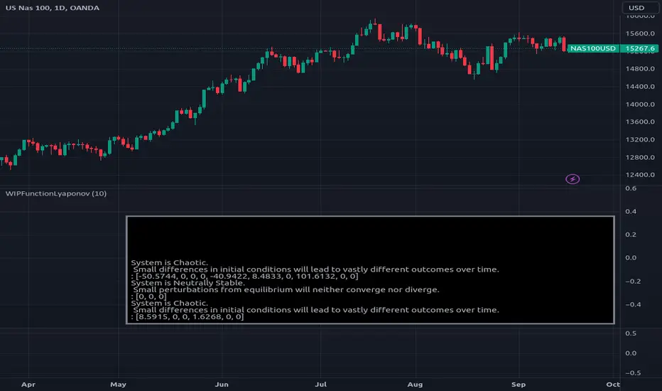
Stability

WIPFunctionLyaponovLibrary "WIPFunctionLyaponov"
Lyapunov exponents are mathematical measures used to describe the behavior of a system over
time. They are named after Russian mathematician Alexei Lyapunov, who first introduced the concept in the
late 19th century. The exponent is defined as the rate at which a particular function or variable changes
over time, and can be positive, negative, or zero.
Positive exponents indicate that a system tends to grow or expand over time, while negative exponents
indicate that a system tends to shrink or decay. Zero exponents indicate that the system does not change
significantly over time. Lyapunov exponents are used in various fields of science and engineering, including
physics, economics, and biology, to study the long-term behavior of complex systems.
~ generated description from vicuna13b
---
To calculate the Lyapunov Exponent (LE) of a given Time Series, we need to follow these steps:
1. Firstly, you should have access to your data in some format like CSV or Excel file. If not, then you can collect it manually using tools such as stopwatches and measuring tapes.
2. Once the data is collected, clean it up by removing any outliers that may skew results. This step involves checking for inconsistencies within your dataset (e.g., extremely large or small values) and either discarding them entirely or replacing with more reasonable estimates based on surrounding values.
3. Next, you need to determine the dimension of your time series data. In most cases, this will be equal to the number of variables being measured in each observation period (e.g., temperature, humidity, wind speed).
4. Now that we have a clean dataset with known dimensions, we can calculate the LE for our Time Series using the following formula:
λ = log(||M^T * M - I||)/log(||v||)
where:
λ (Lyapunov Exponent) is the quantity that will be calculated.
||...|| denotes an Euclidean norm of a vector or matrix, which essentially means taking the square root of the sum of squares for each element in the vector/matrix.
M represents our Jacobian Matrix whose elements are given by:
J_ij = (∂fj / ∂xj) where fj is the jth variable and xj is the ith component of the initial condition vector x(t). In other words, each element in this matrix represents how much a small change in one variable affects another.
I denotes an identity matrix whose elements are all equal to 1 (or any constant value if you prefer). This term essentially acts as a baseline for comparison purposes since we want our Jacobian Matrix M^T * M to be close to it when the system is stable and far away from it when the system is unstable.
v represents an arbitrary vector whose Euclidean norm ||v|| will serve as a scaling factor in our calculation. The choice of this particular vector does not matter since we are only interested in its magnitude (i.e., length) for purposes of normalization. However, if you want to ensure that your results are accurate and consistent across different datasets or scenarios, it is recommended to use the same initial condition vector x(t) as used earlier when calculating our Jacobian Matrix M.
5. Finally, once we have calculated λ using the formula above, we can interpret its value in terms of stability/instability for our Time Series data:
- If λ < 0, then this indicates that the system is stable (i.e., nearby trajectories will converge towards each other over time).
- On the other hand, if λ > 0, then this implies that the system is unstable (i.e., nearby trajectories will diverge away from one another over time).
~ generated description from airoboros33b
---
Reference:
en.wikipedia.org
www.collimator.ai
blog.abhranil.net
www.researchgate.net
physics.stackexchange.com
---
This is a work in progress, it may contain errors so use with caution.
If you find flaws or suggest something new, please leave a comment bellow.
_measure_function(i)
helper function to get the name of distance function by a index (0 -> 13).\
Functions: SSD, Euclidean, Manhattan, Minkowski, Chebyshev, Correlation, Cosine, Camberra, MAE, MSE, Lorentzian, Intersection, Penrose Shape, Meehl.
Parameters:
i (int)
_test(L)
Helper function to test the output exponents state system and outputs description into a string.
Parameters:
L (float )
estimate(X, initial_distance, distance_function)
Estimate the Lyaponov Exponents for multiple series in a row matrix.
Parameters:
X (map)
initial_distance (float) : Initial distance limit.
distance_function (string) : Name of the distance function to be used, default:`ssd`.
Returns: List of Lyaponov exponents.
max(L)
Maximal Lyaponov Exponent.
Parameters:
L (float ) : List of Lyapunov exponents.
Returns: Highest exponent.
Yield Curve Version 2.55.2Welcome to Yield Curve Version 2.55.2
US10Y-US02Y
* Please read description to help understand the information displayed.
* NOTE - This script requires 1 real time update before accurate information is displayed, therefore WILL NOT display the correct information if the Bond Market is Closed over the Weekend.
* NOTE - When values are changed Via Input setting they do take a bit to display based off all the information that is required to display this script.
**FEATURES**
* Input Features let you view the information the way YOU like via Input Settings
* Displays Current Version Title - Toggleable On/Off via Input Settings - Default On
* Plots the Yield Curve of the Bonds listed (Middle Green and Red Line)
* Displays the Spread for each Bond (Top Green and Red Labels) - Toggleable On/Off via Input Settings - Change Size via Input Settings - Default On
* Displays the current Yield for each Bond (Bottom Green and Red Labels) - Toggleable On/Off via Input Settings - Change Size via Input Settings - Default On - Large Size
* Plots the Average of the Entire Yield Curve (BLUE Line within the Yield Curve) - Toggleable On/Off via Input Settings - Default On
* Displays messages based off Yield Inversions (Orange Text) - Toggleable On/Off via Input Settings - Default On if Applicable
* Displays 2 10 Inversion Warning Message (Orange Text) - Toggleable On/Off via Input Settings - Default On if Applicable
* Plots Column Data at the Bottom that tries to help determine the Stability of the Yield Curve (More information Below about Stability) - Toggleable On/Off via Input Settings - Default On
* Plots the 7,20 and 100 SMA of the STABILITY MAX OVERLOAD (More information Below about Stability Max Overload) - Toggleable On/Off via Input Settings - Default On for 100 SMA , 20 SMA and 7 SMA
* Ability to Display Indicator Name and Value via Input Settings - Default On - Displays Stability Max Overload SMA Labels. Toggleable to Non SMA Values. See Below.
**Bottom Columns are all about STABILITY**
* I have tried to come up with an algorithm that helps understand the Stability of the Yield Curve. There are 3 Sections to the Bottom Columns.
* Section 1 - STABILITY (Displayed as the lightest Green or Red Column) Values range from 0 to 1 where 1 equals the MOST UNSTABLE Curve and 0 equals the MOST STABLE Curve
* Section 2 - STABILITY OVERLOAD (Displayed just above the Stability Column a shade darker Green or Red Column)
* Section 3 - STABILITY MAX OVERLOAD (Displayed just above the Stability Overload Column a shade darker Green or Red Column)
What this section tries to do is help understand the Stability of the Curve based on the inversions data. Lower values represent a MORE STABLE curve. If the Yield Curve currently has 0 Inversions all Stability factors should equal 0 and therefore not plot any lower columns. As the Yield Curve becomes more inverted each section represents a value based off that data. GREEN columns represent a MORE Stable Curve from the resolution prior and vise versa.
(S SO SMO)
STABILITY - tests the current Stability of the Curve itself again ranging from 0 to 1 where 0 equals the MOST Stable Curve and 1 equals the MOST Unstable Curve.
STABILIY OVERLOAD - adds a value to STABLITY based off STABILITY itself.
STABILITY MAX OVERLOAD - adds the Entire value to STABILITY derived again from STABILITY.
This section also allows us to see the 7,20 and 100 SMA of the STABILITY MAX OVERLOAD which should always be the GREATEST of ALL STABILTY VALUES.
*Indicator Labels How to use*
Indicator Labels by default are turned On and will display Name and Value Labels for Stability Max Overload SMA values. To switch to (S SO SMO) Labels, toggle "Indicator Labels / SMO SMA Labels", via Input Settings. This button allows you to switch between the two Indicator Label Display options. You must have "Indicators" turned On to view the Labels and therefore is turned On by Default. To turn all of the Indicator Labels Off, simply disable "Indicators" via Input Settings.
Remember - All information displayed can be tuned On or Off besides the Curve itself. There are also other Features Accessible Via the Input Settings.
I will continue to update this script as there is more information I would like to gather and display!
I hope you enjoy,
OpptionsOnly
