Gann Spiral / Square of 9The Gann Spiral, more commonly known as the Square of 9 is one of the most well known tools that Gann used. Today, it is most commonly used to find possible support and resistance levels, and possible reversals in time.
This indicator is a more flexible version of the traditional Gann Spiral / Square. This is achieved by allowing you to change:
Price and Time direction
The timeframe
How often to draw lines based on degrees
Toggles for Price and Time
Price and Time line customization
How to use:
1 - Select your desired starting value of Price and Time.
2 - Choose the direction of Price and Time.
3 - Choose the amount of lines to display.
4 - Choose how often for lines to be drawn (Rotation Degree Value).
==================================================================
Side Note:
This uses a more proper and more accurate formula to "navigate the square". (Sqr x + 2)^2 is not the formula used, but rather (Sqr x + 1)^2.
If you wish to use the formula you're used to, change Full Revolution Value to 180.
The reasoning behind this formula change is because I re-created the square in the form of an actual spiral. The issue with such a conversion is that the formula used to construct it uses one Pi. If you understand circles, you should know that we're off by 180 degrees. A full rotation is 360, not 180.
Correcting for this error requires a slight but important change in the formula, that being +1 instead of +2. This not only corrects it to fit for a proper spiral, but also makes it easier to use fractions. 1/360 results in 1 degree. This slight formula change makes it incompatible when used on the actual Square of 9, however it is technically the more accurate formula.
스크립트에서 "technical"에 대해 찾기

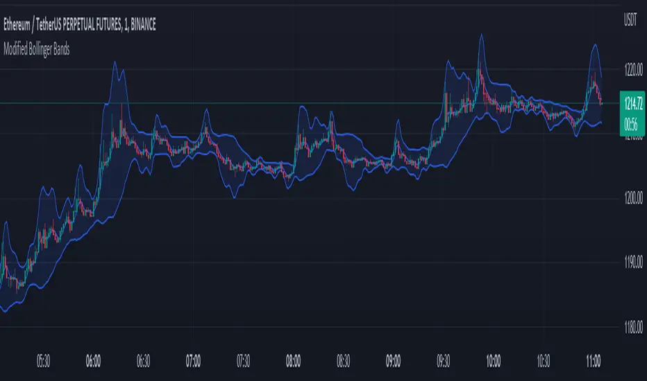
Modified Bollinger BandsThis script has been distributed for learning purposes.
A particular kind of price envelope is "Bollinger Bands" indicator. Upper and lower price range levels are determined by price envelopes. By default, Bollinger Bands are plotted in Tradingview as envelopes at a standard deviation level above and below the price's simple moving average (SMA). I attempted to modify the indicator in this version by adding several kinds of moving averages first. The key feature is that standard deviation should be modified. in Tradingview, SMA calculates the standard deviation. The allocated moving average should be used to calculate the std function when the base line is changed.
Musashi_Katana=== Musashi-Katana ===
This tool was designed to fit my particular trading style and personal theories about the "Alchemy of the markets" and ''Harmonic Structure'.
Context
When following a Technical approach to to surf the markets, there are teachings that must be understood before reaching a confort-zone, this usually happen the possible worst way by constant experimentation, it hurts.
Here few technical hints:
- Align High timeframes with lower timeframes:
This simple concept relax a lot complexity of finding of a trend bias. Musashi-Katana allows you to use technical indicator corresponding to specific timeframes, like daily weekly or yearly. They wont change when you change the chart's timeframe, its very useful as you know where you're standing in the long term, Its quite relaxing.
- Use volume:
The constant usage of volume will allow you to sync with the market's breathing. This shows you the mass of money flowing into and out of the market, is key if you want to understand momentum. This tool can help here, as it have multi-period vwaps. You can use yearly, monthly for swing trading, and even weekly if you enjoy scalping.
Useful stuff:
- You have access to baselines, AMA and Kijun-sen with the possibility of adding ATR bands.
- AMAs come as two lines strategies for different approaches, fast medium or slow.
- You can experiment with normal and multi timeframe moving averages and other trend tools.
Final Note
If used correctly Musashi-Katana is a very powerful tool, which makes no sense as there is no correct usage. Don't add everything at the same time, experiment, combine stuff, every market is different.
Backtest every possible strategy before using it, see what works and doesn't. This gives you a lot of peace, specially while you're at the tip of the spear surfing the markets
--> I personally use this in combination with 'Musashi_Slasher (Mometum+Volatility)', as it gives me volatility and momentum in a very precise way.

[blackcat] L2 Handicap Volume for StocksLevel 2
Background
Handicap volume is a way to understand market logic.
Function
I have studied many classic trading textbooks about volume. Most textbooks tell me that the most authentic indicator in the world is the trading volume, because other things can be faked, but the trading volume is real, and the real money is there, so it cannot be faked! But now, almost everyone knows that if you place an order there, and then eat it yourself, and the volume comes out, it does not reflect the real long-short will of the market.
So why is volume still considered the most important technical indicator by many successful traders in the stock market? Here is to distinguish from the duration and intensity of the trading volume, the actions of the main whales. It's like in the sea, small fish and shrimp can only create ripples, while whales can set off huge waves. When you need to fish, you must go to the sea with both ripples and huge waves. If the volume of a stock or a currency can fluctuate evenly or pulse ECG, the price will move unnaturally, and it will also be small fluctuations or ECG. This corresponds to a group of small fish and shrimp retail investors gathering, or stocks or altcoins with high control of whales, these two cannot participate. Otherwise, either your money will be wasted there, or you will be taken over by the unscrupulous project party with high control area.
This technical indicator is the handicap trading volume and turnover rate indicators. You can see clearly the type of funds operating on this target in a suitable time period, and thus determine whether this target is in line with your trading style and whether you want to participate Among them and so on.
My technical indicator is mainly to clearly see whether there are main whales participating in the stock by distinguishing the trading volume and the enlarged turnover rate. Its main purpose is to judge the character of the stock, that is, the nature of the stock. And in the yellow and purple positions with high turnover rates, it prompts the behavior of the main whales. This is just a reminder. As for whether the main whale will attack or retreat, you need to conduct an in-depth analysis based on market logic. This analysis data has gone beyond the scope of ordinary candle chart analysis, and requires additional dimensions of information to assist judgment.
Remarks
Feedbacks are appreciated.

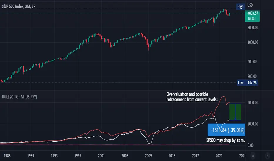
Rule Of 20 - Fair Value Estimation by Inflation & Earnings (TG)The Rule Of 20 is a heuristic calculation to find the fair value of an asset or market given its earnings and current inflation.
Its calculation is straightforward: the fair multiple of the price or price-to-earnings ratio of a stock should be 20 minus the rate of inflation.
In math terms: fair_price-to-earnings_ratio = (20 - inflation) ; fair_value = current_price * fair_price-to-earnings_ratio / real_price-to-earnings_ratio
For example, if a stock or index was trading on 11 times earnings and inflation was 2%, then the theory would be that the fair price-to-earnings ratio would be 20-2 = 18, which is much higher than the real price-to-earnings ratio of 11, and hence the asset would be undervalued.
Conversely, a market or company that was trading on 18 times price-to-earnings ration when inflation was 8% was seen as overvalued, because of the fair price-to-earnings ratio being 20-8=12, hence much lower than the real price-to-earnings ratio of 18.
We can then project the delta between the fair PE and real PE onto the asset's value to obtain the projected fair value, which may be a target of future value the asset may reach or hover around.
For example, as of 1st November 2022, SPX stood at 3871.97, with a PE ratio of 20.14 and an inflation in the US of 7.70. Using the Rule Of 20, we find that the fair PE ratio is 20-7.7=12.3, which is much lower than the current PE ratio of 20.14 by 39%! This may indicate a future possibility of a further downside risk by 39% from current valuation levels.
The origins of this rule are unknown, although the legendary US fund manager Peter Lynch is said to have been an active proponent when he was directing the Fidelity’s Magellan fund from 1977 to 1990.
For more infos about the Rule Of 20, reading this article is recommended: www.sharesmagazine.co.uk
This indicator implements the Rule Of 20 on any asset where the Financials are availble to TradingView, and also for the entire SP:SPX index as a way to assess the wider US stock market. Technically, the calculation is a bit different for the latter, as we cannot access earnings of SPX through Financials on TradingView, so we access it using the QUANDL:MULTPL/SP500_PE_RATIO_MONTH ticker instead.
By default are displayed:
current asset value in red
fair asset value according to the Rule Of 20 in white for SPX, or different shades of purple/maroon for other assets. Note that for SPX there is only one calculation, whereas for other assets there are multiple different ways to calculate earnings, so different fair values can be computed.
fair price-to-earnings ratio (PE ratio) in light grey.
real price-to-earnings ratio in darker grey.
This indicator can be used on SP:SPX ticker, and on most NASDAQ:* tickers, since they have Financials integrated in TradingView. Stocks tickers from other exchanges may not provide Financials data, so this indicator won't work then. If this happens, try to find the same ticker on NASDAQ instead.
Note that by default, only the US stock market is considered. If you want to consider stocks or assets in other regions of the world, please change the inflation ticker to a ticker that reflect the target region's inflation.
Also adding a table to ease interpretation was considered, but then the Timeframe MTF parameter would not work, and since the big advantage of this indicator is to allow for historical comparisons, the table was dropped.
Enjoy, and keep in mind that all models are wrong, but some are useful.
Trade safely!
TG
FluidTrades - SMC Lite
Price action and supply and demand is a key strategy use in trading. We wanted it to be easy and efficient for user to identify these zones, so the user can focus less on marking up charts and focus more on executing trades.
This indicator shows you supply and demand zones by using pivot points to show you the recent highs and the recent lows.
Features
This indicator includes some features relevant to SMC , these are highlighted below:
Full internal & swing market structure labeling in real-time
Swing Structure: Displays the swing structure labels & solid lines on the chart (BOS).
Supply & demand ( bullish & bearish )
Swing Points: Displays swing points labels on chart such as HH, HL, LH, LL.
Options to style the indicator to more easily display these concepts
White OB (supply): search for short opportunities
Blue OB (demand): search for long opportunities
Break of structure ( BOS )
For markets to move up and down a break in market structure must occur. A break in market structure occurs when the market begins to shift direction and break the previous HH and HL or HL and LL of the market. We also integrated the feature that you can see the BOS lines. In the indicator settings you can adjust the color of the label.
Settings
SwingHigh/Low Length: Allows the user to select Historical (default) or Present, which displays only recent data on the chart.
Supply/demand box width: Allows user to change the size of the supply and demand box
History to keep: allows the user to select how many most recent supply & demand box appear on the chart.
Visual settings
Show zig zag : allow user to see market patters within the market
Show price action labels: allow user to turn on/off the (swing points)
Supply box color : allow users to change the color of their supply box
Demand box color : allow users to change the color of their supply box
Bos label color : allow users to change the color of their BOS label
Poi label color : allow user to change the color of their POI label
Price action label : allow users to change the color of their swing points labels
Zig zag color : allow users to change the color of the zig/zag market patters
Warning
Never blindly take a trade on a supply/demand box - wait for a proper market structure to occur before considering a trade.

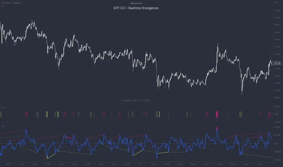
MTF CCI + Realtime DivergencesMulti-timeframe Commodity Channel Index (CCI) + Realtime Divergences + Alerts
This version of the CCI includes the following features:
- Optional 2x sets of triple-timeframe overbought and oversold signals with fully configurable timeframes and overbought and oversold thresholds, can indicate where 3 selected timeframes are all overbought or all oversold at the same time, with alert option.
- Optional divergence lines drawn directly onto the oscillator in realtime, with alert options.
- Configurable pivot periods to fine tune the divergences drawn in order to suit different trading styles and timeframes, including the ability to enable automatic adjustment of pivot period per chart timeframe.
- Alternate timeframe feature allows you to configure the oscillator to use data from a different timeframe than the chart it is loaded on.
- 'Hide oscillator' feature allows traders to hide the oscillator itself, leaving only the background colours indicating the overbought and oversold periods and/or MTF overbought and oversold confluences, as seen in the chart image.
- Also includes standard configurable CCI options, including CCI length and source type. Defaults set to length 20, and hlc3 source type.
- Optional Flip oscillator feature, allows users to flip the oscillator upside down, for use with Tradingviews 'Flip chart' feature (Alt+i), for the purpose of manually spotting divergences, where the trader has a strong natural bias in one direction, so that they can flip both the chart and the oscillator.
- Optional 'Fade oscillator' feature, which will fade out all but the most recent period, reducing visual noise on the chart.
While this version of the CCI has the ability to draw divergences in realtime along with related alerts so you can be notified as divergences occur without spending all day watching the charts, the main purpose of this indicator was to provide the triple-timeframe overbought and oversold confluence signals, in an attempt to add more confluence, weight and reliability to the single timeframe overbought and oversold states, commonly used for trade entry confluence. It's primary purpose is intended for scalping reversal trades on lower timeframes, typically between 1-15 minutes, which can be used in conjunction with the regular divergences the indicator can highlight. The triple timeframe overbought can often indicate near term reversals to the downside, with the triple timeframe oversold often indicating neartime reversals to the upside. The default timeframes for this confluence are set to check the 1m, 5m and 15m timeframes together, ideal for scalping the < 15 minute charts. The default settings for the MTF #1 timeframes (1m, 5m and 15m) are best used on a <5 minute chart.
Its design and use case is based upon the original MTF Stoch RSI + Realtime Divergences found here .
Commodity Channel Index (CCI)
Investopedia has described the popular oscillator as follows:
“The Commodity Channel Index (CCI) is a momentum-based oscillator used to help determine when an investment vehicle is reaching a condition of being overbought or oversold.
Developed by Donald Lambert, this technical indicator assesses price trend direction and strength, allowing traders to determine if they want to enter or exit a trade, refrain from taking a trade, or add to an existing position. In this way, the indicator can be used to provide trade signals when it acts in a certain way.”
You can read more about the CCI, its use cases and calculations here .
How do traders use overbought and oversold levels in their trading?
The oversold level, that is traditionally when the CCI is above the 100 level is typically interpreted as being 'overbought', and below the -100 level is typically considered 'oversold'. Traders will often use the CCI at an overbought level as a confluence for entry into a short position, and the CCI at an oversold level as a confluence for an entry into a long position. These levels do not mean that price will necessarily reverse at those levels in a reliable way, however. This is why this version of the CCI employs the triple timeframe overbought and oversold confluence, in an attempt to add a more confluence and reliability to this usage of the CCI. While traditionally, the overbought and oversold levels are below -100 for oversold, and above 100 for overbought, he default threshold settings of this indicator have been increased to provide fewer, stronger signals, especially suited to the low timeframes and highly volatile assets.
What are divergences?
Divergence is when the price of an asset is moving in the opposite direction of a technical indicator, such as an oscillator, or is moving contrary to other data. Divergence warns that the current price trend may be weakening, and in some cases may lead to the price changing direction.
There are 4 main types of divergence, which are split into 2 categories;
regular divergences and hidden divergences. Regular divergences indicate possible trend reversals, and hidden divergences indicate possible trend continuation.
Regular bullish divergence: An indication of a potential trend reversal, from the current downtrend, to an uptrend.
Regular bearish divergence: An indication of a potential trend reversal, from the current uptrend, to a downtrend.
Hidden bullish divergence: An indication of a potential uptrend continuation.
Hidden bearish divergence: An indication of a potential downtrend continuation.
How do traders use divergences in their trading?
A divergence is considered a leading indicator in technical analysis , meaning it has the ability to indicate a potential price move in the short term future.
Hidden bullish and hidden bearish divergences, which indicate a potential continuation of the current trend are sometimes considered a good place for traders to begin, since trend continuation occurs more frequently than reversals, or trend changes.
When trading regular bullish divergences and regular bearish divergences, which are indications of a trend reversal, the probability of it doing so may increase when these occur at a strong support or resistance level . A common mistake new traders make is to get into a regular divergence trade too early, assuming it will immediately reverse, but these can continue to form for some time before the trend eventually changes, by using forms of support or resistance as an added confluence, such as when price reaches a moving average, the success rate when trading these patterns may increase.
Typically, traders will manually draw lines across the swing highs and swing lows of both the price chart and the oscillator to see whether they appear to present a divergence, this indicator will draw them for you, quickly and clearly, and can notify you when they occur.
Setting alerts.
With this indicator you can set alerts to notify you when any/all of the above types of divergences occur, on any chart timeframe you choose, and also when the triple timeframe overbought and oversold confluences occur.
Configurable pivot period.
You can adjust the default pivot period values to suit your prefered trading style and timeframe. If you like to trade a shorter time frame, lowering the default lookback values will make the divergences drawn more sensitive to short term price action. By default, this indicator has enabled the automatic adjustment of the pivot periods for 4 configurable timeframes, in a bid to optimise the divergences drawn when the indicator is loaded onto any of the 4 timeframes. These timeframes and the auto adjusted pivot periods on each of them can also be reconfigured within the settings menu.
Disclaimer: This script includes code adapted from the Divergence for Many Indicators v4 by LonesomeTheBlue . With special thanks.
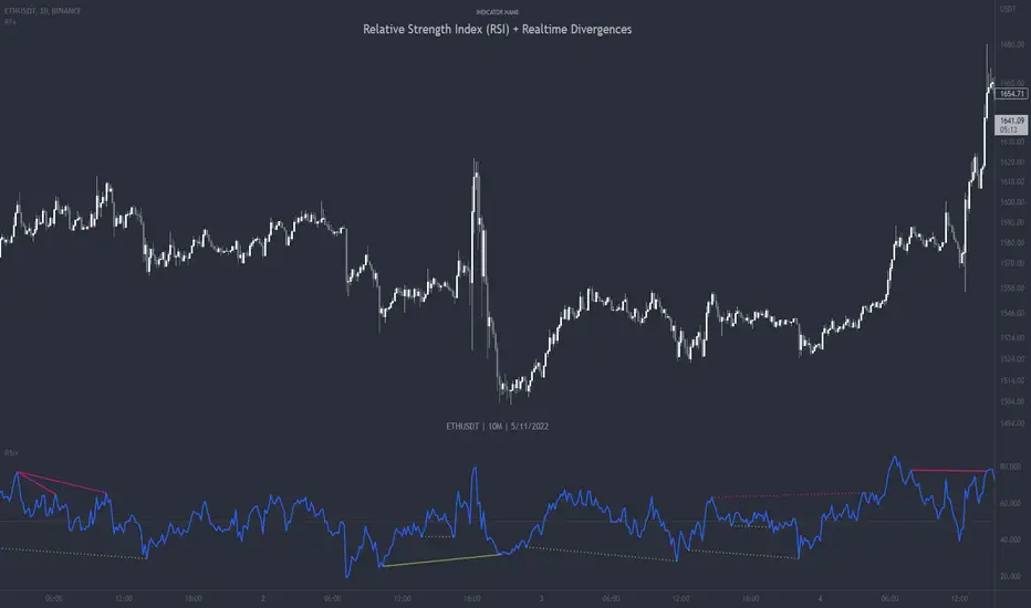
Relative Strength Index (RSI) + Realtime DivergencesRelative Strength Index (RSI) + Realtime Divergences
This version of the RSI indicator includes the following features:
- Optional divergence lines drawn directly onto the oscillator in realtime.
- Configurable alerts to notify you when divergences occur.
- Configurable lookback periods to fine tune the divergences drawn in order to suit different trading styles and timeframes.
- Background colouring option to indicate when the RSI oscillator has crossed above or below its centerline.
- Alternate timeframe feature allows you to configure the oscillator to use data from a different timeframe than the chart it is loaded on.
- Fadeout oscillator feature will fade out all but the most recent history, leaving your chart free of visual noise.
- Flip oscillator feature can be used with the Tradingview 'Flip chart' feature (Alt+i) in order to flip both the chart and the oscillator, too. This feature is to help traders manually spot divergences that may have a strong natural bias in one direction.
- Optional centerline and range bands.
- Various optional moving average types, bollinger bands etc.
This indicator adds additional features onto the standard RSI whose core calculations remain unchanged. Namely, the configurable option to automatically, quickly and clearly draw divergence lines onto the oscillator for you as they occur in realtime. It also has the addition of unique alerts, so you can be notified when divergences occur without spending all day watching the charts. Furthermore, this version of the RSI comes with configurable lookback periods, which can be configured in order to adjust the sensitivity of the divergences, in order to suit shorter or higher timeframe trading approaches.
What is the Relative Strength Index ( RSI )?
Investopedia describes the Relative Strength Index as follows:
“The relative strength index (RSI) is a momentum indicator used in technical analysis. RSI measures the speed and magnitude of a security's recent price changes to evaluate overvalued or undervalued conditions in the price of that security. The RSI is displayed as an oscillator (a line graph) on a scale of zero to 100. The indicator was developed by J. Welles Wilder Jr. and introduced in his seminal 1978 book, New Concepts in Technical Trading Systems.
The RSI can do more than point to overbought and oversold securities. It can also indicate securities that may be primed for a trend reversal or corrective pullback in price. It can signal when to buy and sell. Traditionally, an RSI reading of 70 or above indicates an overbought situation. A reading of 30 or below indicates an oversold condition.”
The RSI is also commonly used to spot divergences.
You can read more about the RSI and its calculations here
What are divergences?
Divergence is when the price of an asset is moving in the opposite direction of a technical indicator, such as an oscillator, or is moving contrary to other data. Divergence warns that the current price trend may be weakening, and in some cases may lead to the price changing direction.
There are 4 main types of divergence, which are split into 2 categories;
regular divergences and hidden divergences. Regular divergences indicate possible trend reversals, and hidden divergences indicate possible trend continuation.
Regular bullish divergence: An indication of a potential trend reversal, from the current downtrend, to an uptrend.
Regular bearish divergence: An indication of a potential trend reversal, from the current uptrend, to a downtrend.
Hidden bullish divergence: An indication of a potential uptrend continuation.
Hidden bearish divergence: An indication of a potential downtrend continuation.
How do traders use divergences in their trading?
A divergence is considered a leading indicator in technical analysis , meaning it has the ability to indicate a potential price move in the short term future.
Hidden bullish and hidden bearish divergences, which indicate a potential continuation of the current trend are sometimes considered a good place for traders to begin, since trend continuation occurs more frequently than reversals, or trend changes.
When trading regular bullish divergences and regular bearish divergences, which are indications of a trend reversal, the probability of it doing so may increase when these occur at a strong support or resistance level . A common mistake new traders make is to get into a regular divergence trade too early, assuming it will immediately reverse, but these can continue to form for some time before the trend eventually changes, by using forms of support or resistance as an added confluence, such as when price reaches a moving average, the success rate when trading these patterns may increase.
Typically, traders will manually draw lines across the swing highs and swing lows of both the price chart and the oscillator to see whether they appear to present a divergence, this indicator will draw them for you, quickly and clearly, and can notify you when they occur.
Setting alerts.
With this indicator you can set alerts to notify you when any/all of the above types of divergences occur, on any chart timeframe you choose.
Configurable pivot periods.
You can adjust the default pivot periods to suit your prefered trading style and timeframe. If you like to trade a shorter time frame, lowering the default lookback values will make the divergences drawn more sensitive to short term price action.
Disclaimer: This script includes code from the stock RSI by Tradingview as well as the Divergence for Many Indicators v4 by LonesomeTheBlue.
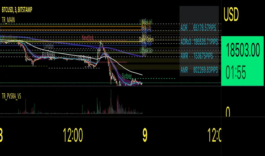
Traders Reality MainThis indicator serves as the Tradingview equivalent of an MT4 indicator suite.
It differentiates from existing TV indicators in its style and total feature set (most notably PVSRA and PVSRA Override)
It was originally designed for forex markets, and it will work for crypto as well, but it has not been tested on stocks.
List of features:
PVSRA Candles
Market boxes (NY/JP/ HK /UK/ FR and Brinks Boxes)
5/13/50/200/800 EMAs (cloud for 50EMA)
Pivot points (S/M/R 1,2,3; PP )
Yesterday and Last Week price range
Average Daily Range (Weekly and Monthly as well)
Daily Open
PVSRA Override
Psychological High/Low
Vector Candle Zones
All of these are configurable in the indicator settings.
Usage instructions:
PVSRA Candle colors meaning:
Green (bull) and red (bear): Candles with volume >= 200% of the average volume of the 10 previous chart candles, and candles where the product of candle spread x candle volume is >= the highest for the 10 previous chart time candles.
Blue (bull) and blue-violet (bear): Candles with volume >= 150% of the average volume of the 10 previous chart candles
PVSRA Override
In order to get reliable bar coloring, we need accurate data. If you're on a chart with low volume on some obscure exchange, you may want to use another exchanges datafeed for the symbol you are on to calculate the PVSRA bar colors with. This lets you do exactly that. By default it's off, but you can turn it on and use INDEX:BTCUSD, or really any other chart you want. You can combine charts too, e.g. use BINANCE:BTCUSDT+COINBASE:BTCUSD.
PVSRA Alerts
Alerts can be made for PVSRA "vector"/"climax" candles:
1. Create Alert (Clock with + sign)
2. Set Condition: "Traders Reality",
3. Select "Alert on Vector Candle",
4. Set it to Once per Bar,
5. choose your notification options.
Market boxes
The market boxes times are configurable and will change depending on the exchange timezone. I recommend to pick your main exchange/chart and adjust the times so that they are correct. Technically you will need to shift the time from the exchanges' timezone to GMT . Default values should be good for UTC based exchanges in current US+UK summer time.
Psychological High/Low
Configurable for Crypto or Forex - draws the perceived Psychological High/Low ranges for the week. Can display historical values too.
Vector Candle Zones
displays unrecovered liquidity left behind on unrecovered vectors. Configurable to take into account candle bodies or candles and wicks.
Recommended additional Tradingview indicator(s):
- TDI - Goldminds, Edited for Market Makers Method by Jakub Donovan
Footnotes
The code was originally by plasmapug, continued development (with permission) is now done by infernix and peshocore and xtech5192 in collaboration with TradersReality.
If you have suggestions or questions, you can message me or leave a comment.
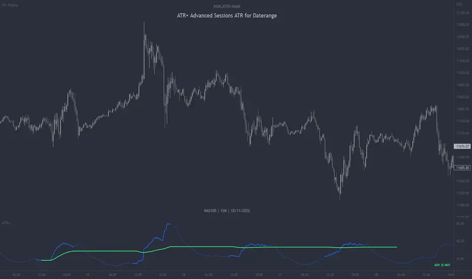
ATR+ Advanced Sessions ATR for DaterangeATR+ Advanced Sessions ATR for Daterange
The ATR+ adds the following additional filters to the stock ATR indicator by Tradingview:
- Calculates the overall average ATR for a user defined daterange, optionally filtered by trading session and selected weekdays, presented as a secondary line over the standard ATR line.
- Basic ATR line, with colour highlight to indicate the selected sessions, days and timeframe being calculated by the average ATR+ line.
- Average ATR+ line indicating the average of all ATRs within the defined timeframe, optionally filtered by instances of a selected trading session and selected weekdays.
- Customisable appearance.
- The ATR+ also includes the basic ATR configuration options typically found in the standard ATR by Tradingview, including period length and smoothing type. Defaults are set to the factory standards: 14 length, RMA smoothing type.
What Is the Average True Range (ATR)?
The ATR is a technical analysis tool that measures market volatility by decomposing the entire range asset price for that period. Investopedia describes the ATR as follows:
"The average true range (ATR) is a technical analysis indicator, introduced by market technician J. Welles Wilder Jr. in his book New Concepts in Technical Trading Systems, that measures market volatility by decomposing the entire range of an asset price for that period.
The true range indicator is taken as the greatest of the following: current high less the current low; the absolute value of the current high less the previous close; and the absolute value of the current low less the previous close. The ATR is then a moving average, generally using 14 days, of the true ranges."
For more information on the ATR and its calculations and use cases, see here:
Investopedia link here.
Tradingview link here.
Note
The indicator may time out if the number of bars being calculated is too long. If this happens, you will need to reduce the datetime range, or increase the chart timeframe in order to reduce the number of bars being calculated and the indicator will attempt to recalculate.
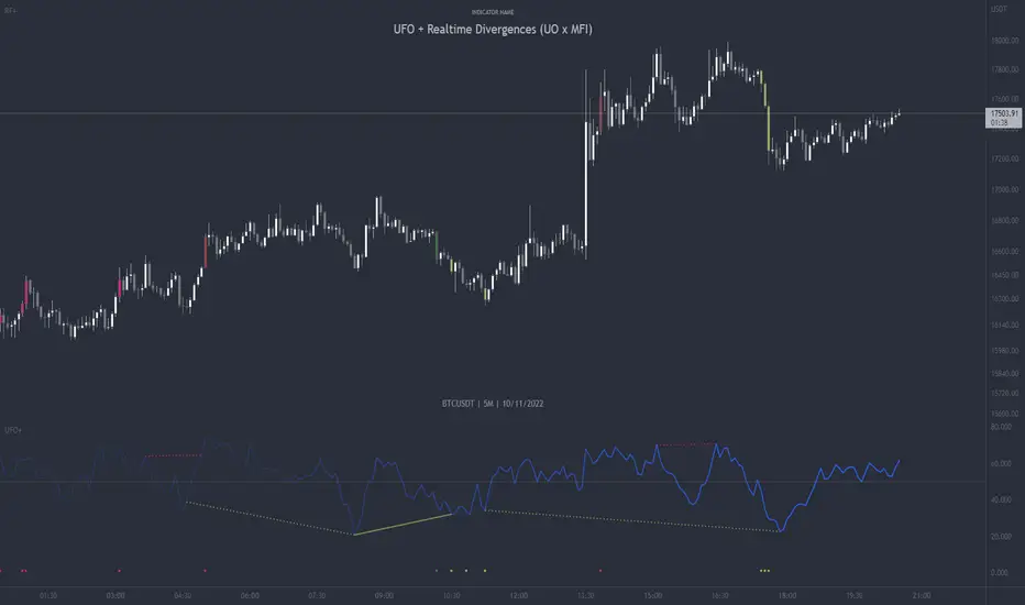
UFO + Realtime Divergences (UO x MFI)UFO + Realtime Divergences (UO x MFI) + Alerts
The UFO is a hybrid of two powerful oscillators - the Ultimate Oscillator (UO) and the Money Flow Index (MFI)
Features of the UFO include:
- Optional divergence lines drawn directly onto the oscillator in realtime.
- Configurable alerts to notify you when divergences occur, as well as centerline crossovers.
- Configurable lookback periods to fine tune the divergences drawn in order to suit different trading styles and timeframes.
- Background colouring option to indicate when the oscillator has crossed its centerline.
- Alternate timeframe feature allows you to configure the oscillator to use data from a different timeframe than the chart it is loaded on.
- 2x MTF triple-timeframe Stochastic RSI overbought and oversold confluence signals painted at the top of the panel for use as a confluence for reversal entry trades.
The core calculations of the UFO+ combine the factory settings of the Ultimate Oscillator and Money Flow Index, taking an average of their combined values for its output eg:
UO_Value + MFI_Value / 2
The result is a powerful oscillator capable of detecting high quality divergences, including on very low timeframes and highly volatile markets, it benefits from the higher weighting of the most recent price action provided by the Ultimate Oscillators calculations, as well as the calculation of the MFI, which incorporates volume data. The UFO and its incorporated 2x triple-timeframe MTF Stoch RSI overbought and oversold signals makes it well adapted for low timeframe scalping and regular divergence trades in particular.
The Ultimate Oscillator (UO)
Tradingview describes the Ultimate Oscillator as follows:
“The Ultimate Oscillator indicator (UO) is a technical analysis tool used to measure momentum across three varying timeframes. The problem with many momentum oscillators is that after a rapid advance or decline in price, they can form false divergence trading signals. For example, after a rapid rise in price, a bearish divergence signal may present itself, however price continues to rise. The Ultimate Oscillator attempts to correct this by using multiple timeframes in its calculation as opposed to just one timeframe which is what is used in most other momentum oscillators.”
You can read more about the UO and its calculations here
The Money Flow Index ( MFI )
Investopedia describes the True Strength Indicator as follows:
“The Money Flow Index ( MFI ) is a technical oscillator that uses price and volume data for identifying overbought or oversold signals in an asset. It can also be used to spot divergences which warn of a trend change in price. The oscillator moves between 0 and 100. Unlike conventional oscillators such as the Relative Strength Index ( RSI ), the Money Flow Index incorporates both price and volume data, as opposed to just price. For this reason, some analysts call MFI the volume-weighted RSI .”
You can read more about the MFI and its calculations here
The Stochastic RSI (relating to the built-in MTF Stoch RSI feature)
The popular oscillator has been described as follows:
“The Stochastic RSI is an indicator used in technical analysis that ranges between zero and one (or zero and 100 on some charting platforms) and is created by applying the Stochastic oscillator formula to a set of relative strength index ( RSI ) values rather than to standard price data. Using RSI values within the Stochastic formula gives traders an idea of whether the current RSI value is overbought or oversold. The Stochastic RSI oscillator was developed to take advantage of both momentum indicators in order to create a more sensitive indicator that is attuned to a specific security's historical performance rather than a generalized analysis of price change.”
You can read more about the Stochastic RSI and its calculations here
How do traders use overbought and oversold levels in their trading?
The oversold level, that is when the Stochastic RSI is above the 80 level is typically interpreted as being 'overbought', and below the 20 level is typically considered 'oversold'. Traders will often use the Stochastic RSI at an overbought level as a confluence for entry into a short position, and the Stochastic RSI at an oversold level as a confluence for an entry into a long position. These levels do not mean that price will necessarily reverse at those levels in a reliable way, however. This is why this version of the Stoch RSI employs the triple timeframe overbought and oversold confluence, in an attempt to add a more confluence and reliability to this usage of the Stoch RSI .
What are divergences?
Divergence is when the price of an asset is moving in the opposite direction of a technical indicator, such as an oscillator, or is moving contrary to other data. Divergence warns that the current price trend may be weakening, and in some cases may lead to the price changing direction.
There are 4 main types of divergence, which are split into 2 categories;
regular divergences and hidden divergences. Regular divergences indicate possible trend reversals, and hidden divergences indicate possible trend continuation.
Regular bullish divergence: An indication of a potential trend reversal, from the current downtrend, to an uptrend.
Regular bearish divergence: An indication of a potential trend reversal, from the current uptrend, to a downtrend.
Hidden bullish divergence: An indication of a potential uptrend continuation.
Hidden bearish divergence: An indication of a potential downtrend continuation.
How do traders use divergences in their trading?
A divergence is considered a leading indicator in technical analysis , meaning it has the ability to indicate a potential price move in the short term future.
Hidden bullish and hidden bearish divergences, which indicate a potential continuation of the current trend are sometimes considered a good place for traders to begin, since trend continuation occurs more frequently than reversals, or trend changes.
When trading regular bullish divergences and regular bearish divergences, which are indications of a trend reversal, the probability of it doing so may increase when these occur at a strong support or resistance level . A common mistake new traders make is to get into a regular divergence trade too early, assuming it will immediately reverse, but these can continue to form for some time before the trend eventually changes, by using forms of support or resistance as an added confluence, such as when price reaches a moving average, the success rate when trading these patterns may increase.
Typically, traders will manually draw lines across the swing highs and swing lows of both the price chart and the oscillator to see whether they appear to present a divergence, this indicator will draw them for you, quickly and clearly, and can notify you when they occur.
Setting alerts.
With this indicator you can set alerts to notify you when any/all of the above types of divergences occur, on any chart timeframe you choose.
Configurable pivot period.
You can adjust the default pivot lookback values to suit your prefered trading style and timeframe. If you like to trade a shorter time frame, lowering the default lookback values will make the divergences drawn more sensitive to short term price action.
Disclaimer: This script includes code from the stock UO and MFI by Tradingview as well as the Divergence for Many Indicators v4 by LonesomeTheBlue.
Big Money Flow & Drift Oscillator [Spiritualhealer117]An easy way to track what big money and market makers are doing in the markets. The Big Money Flow & Drift Oscillator is best suited as a trend indicator, estimating what way the market will drift on low volume and what way it will move on large volume.
This oscillator is composed of two lines, the Big Money Flow and Drift Oscillator. The Big Money Flow line gives the average percentage return of the asset when the volume is greater than the EMA of volume, showing that big money is making moves in the market. The Drift Oscillator gives the average percentage return of the asset when the volume is less than the EMA of volume, where pricing is done by small money and market makers.
By default, between the two lines, there is a color fill, determined based on the following logic:
BMF > drift and BMF > 0: Yellow
drift > BMF and drift > 0: Beige
BMF > drift and BMF < 0: Orange
drift > BMF and drift < 0: Red

[blackcat] L1 Slope OscillatorLevel 1
Background
This technical indicator can judge the upside potential of individual stocks based on the slope
Function
This technical indicator determines whether the trend continues or reverses by defining a fast slope and a slow slope. If it shows a golden cross to buy at a low level, a dead cross to sell. It can be combined with other types of fast technical indicators to determine the resonance of buying and selling points. The premise of buying stocks is that this indicator has a golden cross and the individual stocks are trending upwards.
Remarks
Feedbacks are appreciated.

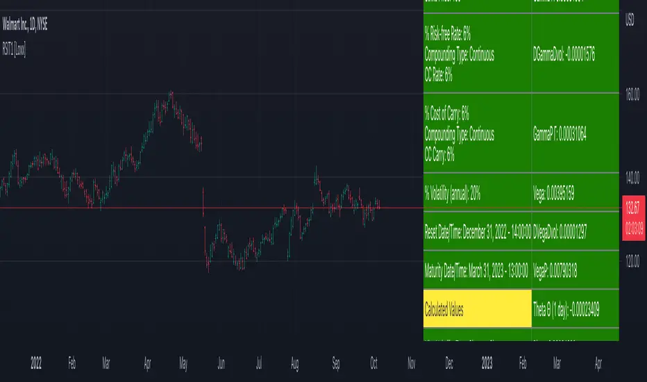
Reset Strike Options-Type 2 (Gray Whaley) [Loxx]For a reset option type 2, the strike is reset in a similar way as a reset option 1. That is, the strike is reset to the asset price at a predetermined future time, if the asset price is below (above) the initial strike price for a call (put). The payoff for such a reset call is max(S - X, 0), and max(X - S, 0) for a put, where X is equal to the original strike X if not reset, and equal to the reset strike if reset. Gray and Whaley (1999) have derived a closed-form solution for the price of European reset strike options. The price of the call option is then given by (via "The Complete Guide to Option Pricing Formulas")
c = Se^(b-r)T2 * M(a1, y1; p) - Xe^(-rT2) * M(a2, y2; p) - Se^(b-r)T1 * N(-a1) * N(z2) * e^-r(T2-T1) + Se^(b-r)T2 * N(-a1) * N(z1)
p = Se^(b-r)T1 * N(a1) * N(-z2) * e^-r(T2-T1) + Se^(b-r)T2 * N(a1) * N(-z1) + Xe^(-rT2) * M(-a2, -y2; p) - Se^(b-r)T2 * M(-a1, -y1; p)
where b is the cost-of-carry of the underlying asset, a is the volatility of the relative price changes in the asset, and r is the risk-free interest rate. K is the strike price of the option, T1 the time to reset (in years), and T2 is its time to expiration. N(x) and M(a,b; p) are, respectively, the univariate and bivariate cumulative normal distribution functions. Further
a1 = (log(S/X) + (b+v^2/2)T1) / v*T1^0.5 ... a2 = a1 - v*T1^0.5
z1 = ((b+v^2/2)(T2-T1)) / v*(T2-T1)^0.5 ... z2 = z1 - v*(T2-T1)^0.5
y1 = (log(S/X) + (b+v^2/2)T1) / v*T1^0.5 ... y2 = a1 - v*T1^0.5
and p = (T1/T2)^0.5. For reset options with multiple reset rights, see Dai, Kwok, and Wu (2003) and Liao and Wang (2003).
Inputs
Asset price ( S )
Strike price ( K )
Reset time ( T1 )
Time to maturity ( T2 )
Risk-free rate ( r )
Cost of carry ( b )
Volatility ( s )
Numerical Greeks or Greeks by Finite Difference
Analytical Greeks are the standard approach to estimating Delta, Gamma etc... That is what we typically use when we can derive from closed form solutions. Normally, these are well-defined and available in text books. Previously, we relied on closed form solutions for the call or put formulae differentiated with respect to the Black Scholes parameters. When Greeks formulae are difficult to develop or tease out, we can alternatively employ numerical Greeks - sometimes referred to finite difference approximations. A key advantage of numerical Greeks relates to their estimation independent of deriving mathematical Greeks. This could be important when we examine American options where there may not technically exist an exact closed form solution that is straightforward to work with. (via VinegarHill FinanceLabs)
Numerical Greeks Outputs
Delta D
Elasticity L
Gamma G
DGammaDvol
GammaP G
Vega
DvegaDvol
VegaP
Theta Q (1 day)
Rho r
Rho futures option r
Phi/Rho2
Carry
DDeltaDvol
Speed
Strike Delta
Strike gamma
Things to know
Only works on the daily timeframe and for the current source price.
You can adjust the text size to fit the screen

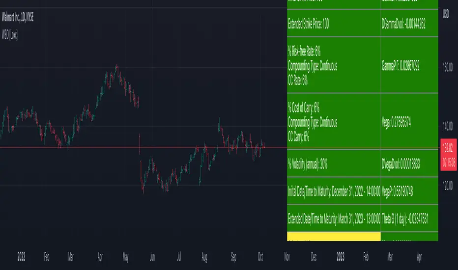
Writer Extendible Option [Loxx]These options can be exercised at their initial maturity date /I but are extended to T2 if the option is out-of-the-money at ti. The payoff from a writer-extendible call option at time T1 (T1 < T2) is (via "The Complete Guide to Option Pricing Formulas")
c(S, X1, X2, t1, T2) = (S - X1) if S>= X1 else cBSM(S, X2, T2-T1)
and for a writer-extendible put is
c(S, X1, X2, T1, T2) = (X1 - S) if S< X1 else pBSM(S, X2, T2-T1)
Writer-Extendible Call
c = cBSM(S, X1, T1) + Se^(b-r)T2 * M(Z1, -Z2; -p) - X2e^-rT2 * M(Z1 - vT^0.5, -Z2 + vT^0.5; -p)
Writer-Extendible Put
p = cBSM(S, X1, T1) + X2e^-rT2 * M(-Z1 + vT^0.5, Z2 - vT^0.5; -p) - Se^(b-r)T2 * M(-Z1, Z2; -p)
b=r options on non-dividend paying stock
b=r-q options on stock or index paying a dividend yield of q
b=0 options on futures
b=r-rf currency options (where rf is the rate in the second currency)
Inputs
Asset price ( S )
Initial strike price ( X1 )
Extended strike price ( X2 )
Initial time to maturity ( t1 )
Extended time to maturity ( T2 )
Risk-free rate ( r )
Cost of carry ( b )
Volatility ( s )
Numerical Greeks or Greeks by Finite Difference
Analytical Greeks are the standard approach to estimating Delta, Gamma etc... That is what we typically use when we can derive from closed form solutions. Normally, these are well-defined and available in text books. Previously, we relied on closed form solutions for the call or put formulae differentiated with respect to the Black Scholes parameters. When Greeks formulae are difficult to develop or tease out, we can alternatively employ numerical Greeks - sometimes referred to finite difference approximations. A key advantage of numerical Greeks relates to their estimation independent of deriving mathematical Greeks. This could be important when we examine American options where there may not technically exist an exact closed form solution that is straightforward to work with. (via VinegarHill FinanceLabs)
Numerical Greeks Output
Delta
Elasticity
Gamma
DGammaDvol
GammaP
Vega
DvegaDvol
VegaP
Theta (1 day)
Rho
Rho futures option
Phi/Rho2
Carry
DDeltaDvol
Speed
Things to know
Only works on the daily timeframe and for the current source price.
You can adjust the text size to fit the screen
Reset Strike Options-Type 1 [Loxx]In a reset call (put) option, the strike is reset to the asset price at a predetermined future time, if the asset price is below (above) the initial strike price. This makes the strike path-dependent. The payoff for a call at maturity is equal to max((S-X)/X, 0) where is equal to the original strike X if not reset, and equal to the reset strike if reset. Similarly, for a put, the payoff is max((X-S)/X, 0) Gray and Whaley (1997) x have derived a closed-form solution for such an option. For a call, we have
c = e^(b-r)(T2-T1) * N(-a2) * N(z1) * e^(-rt1) - e^(-rT2) * N(-a2)*N(z2) - e^(-rT2) * M(a2, y2; p) + (S/X) * e^(b-r)T2 * M(a1, y1; p)
and for a put,
p = e^(-rT2) * N(a2) * N(-z2) - e^(b-r)(T2-T1) * N(a2) * N(-z1) * e^(-rT1) + e^(-rT2) * M(-a2, -y2; p) - (S/X) * e^(b-r)T2 * M(-a1, -y1; p)
where b is the cost-of-carry of the underlying asset, a is the volatil- ity of the relative price changes in the asset, and r is the risk-free interest rate. X is the strike price of the option, r the time to reset (in years), and T is its time to expiration. N(x) and M(a, b; p) are, respec- tively, the univariate and bivariate cumulative normal distribution functions. The remaining parameters are p = (T1/T2)^0.5 and
a1 = (log(S/X) + (b+v^2/2)T1) / vT1^0.5 ... a2 = a1 - vT1^0.5
z1 = (b+v^2/2)(T2-T1)/v(T2-T1)^0.5 ... z2 = z1 - v(T2-T1)^0.5
y1 = log(S/X) + (b+v^2)T2 / vT2^0.5 ... y2 = y1 - vT2^0.5
b=r options on non-dividend paying stock
b=r-q options on stock or index paying a dividend yield of q
b=0 options on futures
b=r-rf currency options (where rf is the rate in the second currency)
Inputs
Asset price ( S )
Initial strike price ( X1 )
Extended strike price ( X2 )
Initial time to maturity ( t1 )
Extended time to maturity ( T2 )
Risk-free rate ( r )
Cost of carry ( b )
Volatility ( s )
Numerical Greeks or Greeks by Finite Difference
Analytical Greeks are the standard approach to estimating Delta, Gamma etc... That is what we typically use when we can derive from closed form solutions. Normally, these are well-defined and available in text books. Previously, we relied on closed form solutions for the call or put formulae differentiated with respect to the Black Scholes parameters. When Greeks formulae are difficult to develop or tease out, we can alternatively employ numerical Greeks - sometimes referred to finite difference approximations. A key advantage of numerical Greeks relates to their estimation independent of deriving mathematical Greeks. This could be important when we examine American options where there may not technically exist an exact closed form solution that is straightforward to work with. (via VinegarHill FinanceLabs)
Numerical Greeks Ouput
Delta
Elasticity
Gamma
DGammaDvol
GammaP
Vega
DvegaDvol
VegaP
Theta (1 day)
Rho
Rho futures option
Phi/Rho2
Carry
DDeltaDvol
Speed
Things to know
Only works on the daily timeframe and for the current source price.
You can adjust the text size to fit the screen
Fade-in Options [Loxx]A fade-in call has the same payoff as a standard call except the size of the payoff is weighted by how many fixings the asset price were inside a predefined range (L, U). If the asset price is inside the range for every fixing, the payoff will be identical to a plain vanilla option. More precisely, for a call option, the payoff will be max(S(T) - X, 0) X 1/n Sum(n(i)), where n is the total number of fixings and n(i) = 1 if at fixing i the asset price is inside the range, and n(i) = 0 otherwise. Similarly, for a put, the payoff is max(X - S(T), 0) X 1/n Sum(n(i)).
Brockhaus, Ferraris, Gallus, Long, Martin, and Overhaus (1999) describe a closed-form formula for fade-in options. For a call the value is given by
max(X - S(T), 0) X 1/n Sum(n(i))
describe a closed-form formula for fade-in options. For a call the value is given by
c = 1/n * Sum(S^((b-r)*T) * (M(-d5, d1; -p) - M(-d3, d1; -p)) - Xe^(-rT) * (M(-d6, d2; -p) - M(-d4, d2; -p))
where n is the number of fixings, p = (t1^0.5/T^0.5), t1 = iT/n
d1 = (log(S/X) + (b + v^2/2)*T) / (v * T^0.5) ... d2 = d1 - v*T^0.5
d3 = (log(S/L) + (b + v^2/2)*t1) / (v * t1^0.5) ... d4 = d3 - v*t1^0.5
d5 = (log(S/U) + (b + v^2/2)*t1) / (v * t1^0.5) ... d6 = d5 - v*t1^0.5
The value of a put is similarly
p = 1/n * Sum(Xe^(-rT) * (M(-d6, -d2; -p) - M(-d4, -d2; -p))) - S^((b-r)*T) * (M(-d5, -d1; -p) - M(-d3, -d1; -p)
b=r options on non-dividend paying stock
b=r-q options on stock or index paying a dividend yield of q
b=0 options on futures
b=r-rf currency options (where rf is the rate in the second currency)
Inputs
Asset price ( S )
Strike price ( K )
Lower barrier ( L )
Upper barrier ( U )
Time to maturity ( T )
Risk-free rate ( r )
Cost of carry ( b )
Volatility ( s )
Fixings ( n )
cnd1(x) = Cumulative Normal Distribution
nd(x) = Standard Normal Density Function
cbnd3() = Cumulative Bivariate Distribution
convertingToCCRate(r, cmp ) = Rate compounder
Numerical Greeks or Greeks by Finite Difference
Analytical Greeks are the standard approach to estimating Delta, Gamma etc... That is what we typically use when we can derive from closed form solutions. Normally, these are well-defined and available in text books. Previously, we relied on closed form solutions for the call or put formulae differentiated with respect to the Black Scholes parameters. When Greeks formulae are difficult to develop or tease out, we can alternatively employ numerical Greeks - sometimes referred to finite difference approximations. A key advantage of numerical Greeks relates to their estimation independent of deriving mathematical Greeks. This could be important when we examine American options where there may not technically exist an exact closed form solution that is straightforward to work with. (via VinegarHill FinanceLabs)
Things to know
Only works on the daily timeframe and for the current source price.
You can adjust the text size to fit the screen

Log Contract Ln(S/X) [Loxx]A log contract, first introduced by Neuberger (1994) and Neuberger (1996), is not strictly an option. It is, however, an important building block in volatility derivatives (see Chapter 6 as well as Demeterfi, Derman, Kamal, and Zou, 1999). The payoff from a log contract at maturity T is simply the natural logarithm of the underlying asset divided by the strike price, ln(S/ X). The payoff is thus nonlinear and has many similarities with options. The value of this contract is (via "The Complete Guide to Option Pricing Formulas")
L = e^(-r * T) * (log(S/X) + (b-v^2/2)*T)
The delta of a log contract is
delta = (e^(-r*T) / S)
and the gamma is
gamma = (e^(-r*T) / S^2)
Inputs
S = Stock price.
K = Strike price of option.
T = Time to expiration in years.
r = Risk-free rate
c = Cost of Carry
V = Variance of the underlying asset price
cnd1(x) = Cumulative Normal Distribution
nd(x) = Standard Normal Density Function
convertingToCCRate(r, cmp ) = Rate compounder
Numerical Greeks or Greeks by Finite Difference
Analytical Greeks are the standard approach to estimating Delta, Gamma etc... That is what we typically use when we can derive from closed form solutions. Normally, these are well-defined and available in text books. Previously, we relied on closed form solutions for the call or put formulae differentiated with respect to the Black Scholes parameters. When Greeks formulae are difficult to develop or tease out, we can alternatively employ numerical Greeks - sometimes referred to finite difference approximations. A key advantage of numerical Greeks relates to their estimation independent of deriving mathematical Greeks. This could be important when we examine American options where there may not technically exist an exact closed form solution that is straightforward to work with. (via VinegarHill FinanceLabs)
Things to know
Only works on the daily timeframe and for the current source price.
You can adjust the text size to fit the screen
Log Option [Loxx]A log option introduced by Wilmott (2000) has a payoff at maturity equal to max(log(S/X), 0), which is basically an option on the rate of return on the underlying asset with strike log(X). The value of a log option is given by: (via "The Complete Guide to Option Pricing Formulas")
e^−rT * n(d2)σ√(T − t) + e^−rT*(log(S/K) + (b −σ^2/2)T) * N(d2)
where N(*) is the cumulative normal distribution function, n(*) is the normal density function, and
d = ((log(S/X) + (b - v^2/2)*T) / (v*T^0.5)
b=r options on non-dividend paying stock
b=r-q options on stock or index paying a dividend yield of q
b=0 options on futures
b=r-rf currency options (where rf is the rate in the second currency)
Inputs
S = Stock price.
K = Strike price of option.
T = Time to expiration in years.
r = Risk-free rate
c = Cost of Carry
V = Variance of the underlying asset price
cnd1(x) = Cumulative Normal Distribution
nd(x) = Standard Normal Density Function
convertingToCCRate(r, cmp ) = Rate compounder
Numerical Greeks or Greeks by Finite Difference
Analytical Greeks are the standard approach to estimating Delta, Gamma etc... That is what we typically use when we can derive from closed form solutions. Normally, these are well-defined and available in text books. Previously, we relied on closed form solutions for the call or put formulae differentiated with respect to the Black Scholes parameters. When Greeks formulae are difficult to develop or tease out, we can alternatively employ numerical Greeks - sometimes referred to finite difference approximations. A key advantage of numerical Greeks relates to their estimation independent of deriving mathematical Greeks. This could be important when we examine American options where there may not technically exist an exact closed form solution that is straightforward to work with. (via VinegarHill FinanceLabs)
Things to know
Only works on the daily timeframe and for the current source price.
You can adjust the text size to fit the screen
Log Contract Ln(S) [Loxx]A log contract, first introduced by Neuberger (1994) and Neuberger (1996), is not strictly an option. It is, however, an important building block in volatility derivatives (see Chapter 6 as well as Demeterfi, Derman, Kamal, and Zou, 1999). The payoff from a log contract at maturity T is simply the natural logarithm of the underlying asset divided by the strike price, ln(S/ X). The payoff is thus nonlinear and has many similarities with options. The value of this contract is (via "The Complete Guide to Option Pricing Formulas")
L = e^(-r * T) * (log(S/X) + (b-v^2/2)*T)
The delta of a log contract is
delta = (e^(-r*T) / S)
and the gamma is
gamma = (e^(-r*T) / S^2)
An even simpler version of the log contract is when the payoff simply is ln(S). The payoff is clearly still nonlinear in the underlying asset. It follows that the value of this contract is:
L = e^(-r * T) * (log(S) + (b-v^2/2)*T)
The theta/time decay of a log contract is
theta = - 1/T * v^2
and its exposure to the stock price, delta, is
delta = - 2/T * 1/S
This basically tells you that you need to be long stocks to be delta- neutral at any time. Moreover, the gamma is
gamma = 2 / (T * S^2)
b=r options on non-dividend paying stock
b=r-q options on stock or index paying a dividend yield of q
b=0 options on futures
b=r-rf currency options (where rf is the rate in the second currency)
Inputs
S = Stock price.
T = Time to expiration in years.
r = Risk-free rate
c = Cost of Carry
V = volatility of the underlying asset price
cnd1(x) = Cumulative Normal Distribution
nd(x) = Standard Normal Density Function
convertingToCCRate(r, cmp ) = Rate compounder
Numerical Greeks or Greeks by Finite Difference
Analytical Greeks are the standard approach to estimating Delta, Gamma etc... That is what we typically use when we can derive from closed form solutions. Normally, these are well-defined and available in text books. Previously, we relied on closed form solutions for the call or put formulae differentiated with respect to the Black Scholes parameters. When Greeks formulae are difficult to develop or tease out, we can alternatively employ numerical Greeks - sometimes referred to finite difference approximations. A key advantage of numerical Greeks relates to their estimation independent of deriving mathematical Greeks. This could be important when we examine American options where there may not technically exist an exact closed form solution that is straightforward to work with. (via VinegarHill FinanceLabs)
Things to know
Only works on the daily timeframe and for the current source price.
You can adjust the text size to fit the screen

Powered Option [Loxx]At maturity, a powered call option pays off max(S - X, 0)^i and a put pays off max(X - S, 0)^i . Esser (2003 describes how to value these options (see also Jarrow and Turnbull, 1996, Brockhaus, Ferraris, Gallus, Long, Martin, and Overhaus, 1999). (via "The Complete Guide to Option Pricing Formulas")
b=r options on non-dividend paying stock
b=r-q options on stock or index paying a dividend yield of q
b=0 options on futures
b=r-rf currency options (where rf is the rate in the second currency)
Inputs
S = Stock price.
K = Strike price of option.
T = Time to expiration in years.
r = Risk-free rate
c = Cost of Carry
V = volatility of the underlying asset price
i = power
cnd1(x) = Cumulative Normal Distribution
nd(x) = Standard Normal Density Function
combin(x) = Combination function, calculates the number of possible combinations for two given numbers
convertingToCCRate(r, cmp ) = Rate compounder
Numerical Greeks or Greeks by Finite Difference
Analytical Greeks are the standard approach to estimating Delta, Gamma etc... That is what we typically use when we can derive from closed form solutions. Normally, these are well-defined and available in text books. Previously, we relied on closed form solutions for the call or put formulae differentiated with respect to the Black Scholes parameters. When Greeks formulae are difficult to develop or tease out, we can alternatively employ numerical Greeks - sometimes referred to finite difference approximations. A key advantage of numerical Greeks relates to their estimation independent of deriving mathematical Greeks. This could be important when we examine American options where there may not technically exist an exact closed form solution that is straightforward to work with. (via VinegarHill FinanceLabs)
Things to know
Only works on the daily timeframe and for the current source price.
You can adjust the text size to fit the screen

Capped Standard Power Option [Loxx]Power options can lead to very high leverage and thus entail potentially very large losses for short positions in these options. It is therefore common to cap the payoff. The maximum payoff is set to some predefined level C. The payoff at maturity for a capped power call is min . Esser (2003) gives the closed-form solution: (via "The Complete Guide to Option Pricing Formulas")
c = S^i * (e^((i - 1) * (r + i*v^2 / 2) - i * (r - b))*T) * (N(e1) - N(e3)) - e^(-r*T) * (X*N(e2) - (C + X) * N(e4))
while the value of a put is
e1 = (log(S/X^(1/i)) + (b + (i - 1/2)*v^2)*T) / v*T^0.5
e3 = (log(S/(C + X)^(1/i)) + (b + (i - 1/2)*v^2)*T) / v*T^0.5
e4 = e3 - i * v * T^0.5
In the case of a capped power put, we have
p = e^(-r*T) * (X*N(-e2) - (C + X) * N(-e4)) - S^i * (e^((i - 1) * (r + i*v^2 / 2) - i * (r - b))*T) * (N(-e1) - N(-e3))
where e1 and e2 is as before. e3 and e4 has to be changed to
e3 = (log(S/(X - C)^(1/i)) + (b + (i - 1/2)*v^2)*T) / v*T^0.5
e4 = e3 - i * v * T^0.5
b=r options on non-dividend paying stock
b=r-q options on stock or index paying a dividend yield of q
b=0 options on futures
b=r-rf currency options (where rf is the rate in the second currency)
Inputs
S = Stock price.
K = Strike price of option.
T = Time to expiration in years.
r = Risk-free rate
c = Cost of Carry
V = Variance of the underlying asset price
i = power
c = Capped on pay off
cnd1(x) = Cumulative Normal Distribution
nd(x) = Standard Normal Density Function
convertingToCCRate(r, cmp ) = Rate compounder
Numerical Greeks or Greeks by Finite Difference
Analytical Greeks are the standard approach to estimating Delta, Gamma etc... That is what we typically use when we can derive from closed form solutions. Normally, these are well-defined and available in text books. Previously, we relied on closed form solutions for the call or put formulae differentiated with respect to the Black Scholes parameters. When Greeks formulae are difficult to develop or tease out, we can alternatively employ numerical Greeks - sometimes referred to finite difference approximations. A key advantage of numerical Greeks relates to their estimation independent of deriving mathematical Greeks. This could be important when we examine American options where there may not technically exist an exact closed form solution that is straightforward to work with. (via VinegarHill FinanceLabs)
Things to know
Only works on the daily timeframe and for the current source price.
You can adjust the text size to fit the screen

Standard Power Option [Loxx]Standard power options (aka asymmetric power options) have nonlinear payoff at maturity. For a call, the payoff is max(S^i - X, 0), and for a put, it is max(X - S^i , 0), where i is some power (i > 0). The value of this power call is given by (see Heynen and Kat, 1996c; Zhang, 1998; and Esser, 2003). (via "The Complete Guide to Option Pricing Formulas")
c = S^i * (e^((i - 1) * (r + i*v^2 / 2) - i * (r - b))*T) * N(d1) - X*e^(-r*T) * N(d2)
while the value of a put is
p = X*e^(-r*T) * N(-d2) - S^i * (e^((i - 1) * (r + i*v^2 / 2) - i * (r - b))*T) * N(-d1)
where
d1 = (log(S/X^(1/i)) + (b + (i - 1/2)*v^2)*T) / v*T^0.5
d2 = d1 - i * v * T^0.5
b=r options on non-dividend paying stock
b=r-q options on stock or index paying a dividend yield of q
b=0 options on futures
b=r-rf currency options (where rf is the rate in the second currency)
Inputs
S = Stock price.
K = Strike price of option.
T = Time to expiration in years.
r = Risk-free rate
c = Cost of Carry
V = Variance of the underlying asset price
pwr = power
cnd1(x) = Cumulative Normal Distribution
nd(x) = Standard Normal Density Function
convertingToCCRate(r, cmp ) = Rate compounder
Numerical Greeks or Greeks by Finite Difference
Analytical Greeks are the standard approach to estimating Delta, Gamma etc... That is what we typically use when we can derive from closed form solutions. Normally, these are well-defined and available in text books. Previously, we relied on closed form solutions for the call or put formulae differentiated with respect to the Black Scholes parameters. When Greeks formulae are difficult to develop or tease out, we can alternatively employ numerical Greeks - sometimes referred to finite difference approximations. A key advantage of numerical Greeks relates to their estimation independent of deriving mathematical Greeks. This could be important when we examine American options where there may not technically exist an exact closed form solution that is straightforward to work with. (via VinegarHill FinanceLabs)
Things to know
Only works on the daily timeframe and for the current source price.
You can adjust the text size to fit the screen
