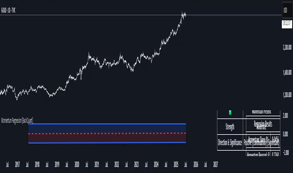
Momentum Regression [BackQuant]Momentum Regression
The Momentum Regression is an advanced statistical indicator built to empower quants, strategists, and technically inclined traders with a robust visual and quantitative framework for analyzing momentum effects in financial markets. Unlike traditional momentum indicators that rely on raw price movements or moving averages, this tool leverages a volatility-adjusted linear regression model (y ~ x) to uncover and validate momentum behavior over a user-defined lookback window.
Purpose & Design Philosophy
Momentum is a core anomaly in quantitative finance — an effect where assets that have performed well (or poorly) continue to do so over short to medium-term horizons. However, this effect can be noisy, regime-dependent, and sometimes spurious.
The Momentum Regression is designed as a pre-strategy analytical tool to help you filter and verify whether statistically meaningful and tradable momentum exists in a given asset. Its architecture includes:
Volatility normalization to account for differences in scale and distribution.
Regression analysis to model the relationship between past and present standardized returns.
Deviation bands to highlight overbought/oversold zones around the predicted trendline.
Statistical summary tables to assess the reliability of the detected momentum.
Core Concepts and Calculations
The model uses the following:
Independent variable (x): The volatility-adjusted return over the chosen momentum period.
Dependent variable (y): The 1-bar lagged log return, also adjusted for volatility.
A simple linear regression is performed over a large lookback window (default: 1000 bars), which reveals the slope and intercept of the momentum line. These values are then used to construct:
A predicted momentum trendline across time.
Upper and lower deviation bands , representing ±n standard deviations of the regression residuals (errors).
These visual elements help traders judge how far current returns deviate from the modeled momentum trend, similar to Bollinger Bands but derived from a regression model rather than a moving average.
Key Metrics Provided
On each update, the indicator dynamically displays:
Momentum Slope (β₁): Indicates trend direction and strength. A higher absolute value implies a stronger effect.
Intercept (β₀): The predicted return when x = 0.
Pearson’s R: Correlation coefficient between x and y.
R² (Coefficient of Determination): Indicates how well the regression line explains the variance in y.
Standard Error of Residuals: Measures dispersion around the trendline.
t-Statistic of β₁: Used to evaluate statistical significance of the momentum slope.
These statistics are presented in a top-right summary table for immediate interpretation. A bottom-right signal table also summarizes key takeaways with visual indicators.
Features and Inputs
✅ Volatility-Adjusted Momentum : Reduces distortions from noisy price spikes.
✅ Custom Lookback Control : Set the number of bars to analyze regression.
✅ Extendable Trendlines : For continuous visualization into the future.
✅ Deviation Bands : Optional ±σ multipliers to detect abnormal price action.
✅ Contextual Tables : Help determine strength, direction, and significance of momentum.
✅ Separate Pane Design : Cleanly isolates statistical momentum from price chart.
How It Helps Traders
📉 Quantitative Strategy Validation:
Use the regression results to confirm whether a momentum-based strategy is worth pursuing on a specific asset or timeframe.
🔍 Regime Detection:
Track when momentum breaks down or reverses. Slope changes, drops in R², or weak t-stats can signal regime shifts.
📊 Trade Filtering:
Avoid false positives by entering trades only when momentum is both statistically significant and directionally favorable.
📈 Backtest Preparation:
Before running costly simulations, use this tool to pre-screen assets for exploitable return structures.
When to Use It
Before building or deploying a momentum strategy : Test if momentum exists and is statistically reliable.
During market transitions : Detect early signs of fading strength or reversal.
As part of an edge-stacking framework : Combine with other filters such as volatility compression, volume surges, or macro filters.
Conclusion
The Momentum Regression indicator offers a powerful fusion of statistical analysis and visual interpretation. By combining volatility-adjusted returns with real-time linear regression modeling, it helps quantify and qualify one of the most studied and traded anomalies in finance: momentum.
스크립트에서 "technical"에 대해 찾기
Price Reaction Analysis by Day of WeekOverview
The "Price Reaction Analysis by Day of Week" indicator is a tool that enables traders to analyze historical price reaction patterns to technical indicator signals on a selected day of the week. It examines price behavior on a chosen candle (from 1 to 30) in the next day or subsequent days after a signal, depending on the timeframe, and provides success rate statistics to support data-driven trading decisions. The indicator is optimized for timeframes up to 1 day (e.g., 1D, 12H, 8H, 6H, 4H, 1H, 15M), as the analysis relies on day-of-week comparisons. Lower timeframes generate more signals due to the higher number of candles per day.
Key Features
1. Flexible Technical Indicator Selection
Users can choose one of four technical indicators: RSI, SMI, MA, or Bollinger Bands. Each indicator has configurable parameters, such as:
RSI length, oversold/overbought levels.
SMI length, %K and %D smoothing, signal levels.
MA length.
Bollinger Bands length and multiplier.
2. Day-of-Week Analysis
The indicator allows users to select a day of the week (Monday, Tuesday, Wednesday, Thursday, Friday) for generating signals. It analyzes price reactions on a selected candle (from 1 to 30) in the next day or subsequent days after the signal. Examples:
On a daily timeframe, a signal on Monday can be analyzed for the first, fourth, or later candle (up to 30) in subsequent days (e.g., Tuesday, Wednesday).
On timeframes lower than 1 day (e.g., 12H, 8H, 6H, 4H, 1H, 15M), the analysis targets the selected candle in the next day or subsequent days. For example, on a 4H timeframe, you can analyze the second Tuesday candle following a Monday signal. The maximum timeframe is 1 day to ensure consistent day-of-week analysis.
3. Visual Signals
Signals for the analysis period are marked with background highlights in real-time when the indicator’s conditions are met. The last highlighted candle of the selected day is always analyzed. Arrows are displayed on the chart at the candle specified by the “Candles to Compare” setting (e.g., the first candle if set to 1):
Green upward triangles (below the candle) for successful buy signals (the closing price of the selected candle is higher than the signal candle’s close).
Red downward triangles (above the candle) for successful sell signals (the closing price of the selected candle is lower than the signal candle’s close).
Gray “x” marks for unsuccessful signals (no price reversal in the expected direction). Arrow positions are intuitive: buy signals below the candle, sell signals above. Highlights and arrows do not require waiting for future signals but are essential for calculating statistics.
Note: The first candle of the next day may appear shifted on the chart due to timezone differences, which can affect the timing of signal appearance.
4. Signal Conditions (Highlights) for Each Indicator
RSI: The oscillator is in oversold (buy) or overbought (sell) zones.
SMI: SMI returns from oversold (buy) or overbought (sell) zones.
MA: Price crosses the MA (upward for buy, downward for sell).
Bollinger Bands: Price returns inside the bands (from below for buy, from above for sell).
5. Success Rate Statistics
A table in the top-right corner of the chart displays:
The number of buy and sell signals for the selected day of the week.
The percentage of cases where the price of the selected candle in the next day or subsequent days reversed as expected (e.g., rising after a buy signal). Statistics are based on comparing the closing price of the signal candle with the closing price of the selected candle (e.g., first, fourth) in the next day or subsequent days.
Important: Statistics do not account for price movements within the candle or after its close. The price on the selected candle (e.g., fourth) may be lower than earlier candles but still higher than the signal candle, counting as a positive buy signal, though it does not guarantee profit.
6. Date Range
Users can specify the analysis date range, enabling strategy testing on historical data from a chosen period. Ensure the start and end dates are set correctly.
Applications
The indicator is designed for traders who want to leverage historical patterns for position planning. Examples:
On a 4-hour timeframe: If a sell signal highlight appears on Monday and statistics show an 80% chance that the fourth Tuesday candle is bearish, traders may consider playing a correction at the open of that candle.
On a daily timeframe: If a highlight indicates market overheating, traders may consider entering a position at the open of the first candle after the signal (e.g., Tuesday), provided statistics suggest an edge. Users can analyze the signal on the first candle and check later candles to validate results, increasing confidence in consistent patterns.
Key Settings
Indicator Type: Choose between RSI, SMI, MA, or Bollinger Bands.
Selected Day: Monday, Tuesday, Wednesday, Thursday, or Friday.
Candles to Compare: The number of the candle in the next day or subsequent days (from 1 to 30).
Indicator Parameters: Lengths, levels (e.g., oversold/overbought for RSI).
Background Colors: Configurable highlights for buy and sell signals.
Notes
Timeframes: The indicator is optimized for timeframes up to 1 day (e.g., 1D, 12H, 8H, 6H, 4H, 1H, 15M), as the analysis relies on day-of-week patterns. Timeframes lower than 1 day generate more signals due to the higher number of candles per day.
Candle Shift: The first candle of the next day may appear shifted on the chart due to timezone differences, affecting the timing of signals across markets or platforms.
Statistical Limitations: Results are based on the closing prices of the selected candle, ignoring fluctuations in earlier candles, within the candle, or subsequent price movements. Traders must assess whether entering at the open or after the close of the selected candle is profitable.
Testing: Effectiveness depends on historical data and parameter settings. Testing different configurations across markets and timeframes is recommended.
Who Is It For?
Swing and position traders who base decisions on technical analysis and historical patterns.
Market analysts seeking patterns in price behavior by day of the week.
TradingView users of all experience levels, thanks to an intuitive interface and flexible settings.

Momentum Trail Oscillator [AlgoAlpha]🟠 OVERVIEW
This script builds a Momentum Trail Oscillator designed to measure directional momentum strength and dynamically track shifts in trend bias using a combination of smoothed price change calculations and adaptive trailing bands. The oscillator aims to help traders visualize when momentum is expanding or contracting and to identify transitions between bullish and bearish conditions.
🟠 CONCEPTS
The core idea combines two methods. First, the script calculates a normalized momentum measure by smoothing price changes relative to their absolute values, which creates a bounded oscillator that highlights whether moves are directional or choppy. Second, it uses a trailing band mechanism inspired by volatility stops, where bands adapt to the oscillator’s volatility, adjusting the thresholds that define a shift in directional bias. This dual approach seeks to address both the magnitude and persistence of momentum, reducing false signals in ranging markets.
🟠 FEATURES
The momentum calculation applies Hull Moving Averages and double EMA smoothing to price changes, producing a smooth, responsive oscillator.
The trailing bands are derived by offsetting a weighted moving average of the oscillator by a multiple of recent momentum volatility. A directional state variable tracks whether the oscillator is above or below the bands, updating when the momentum crosses these dynamic thresholds.
Overbought and oversold zones are visually marked between fixed levels (+30/+40 and -30/-40), with color fills to highlight when momentum is in extreme areas. The script plots signals on both the oscillator pane and optionally overlays markers on the main price chart for clarity.
🟠 USAGE
To use the indicator, apply it to any symbol and timeframe. The “Oscillator Length” controls how sensitive the momentum line is to recent price changes—lower values react faster, higher values smooth out noise. The “Trail Multiplier” sets how far the adaptive bands sit from the oscillator mid-line, which affects how often trend state changes occur. When the momentum line rises into the upper filled area and then crosses back below +40, it signals potential overbought exhaustion. The opposite applies for the oversold zone below -40. The plotted trailing bands switch visibility depending on the current directional state: when momentum is trending up, the lower band acts as the active trailing stop, and when trending down, the upper band becomes active. Trend changes are marked with circular symbols when the direction variable flips, and optional overlay arrows appear on the price chart to highlight overbought or oversold reversals. Traders can combine these signals with their own price action or volume analysis to confirm entries or exits.

Multi-Confluence Swing Hunter V1# Multi-Confluence Swing Hunter V1 - Complete Description
Overview
The Multi-Confluence Swing Hunter V1 is a sophisticated low timeframe scalping strategy specifically optimized for MSTR (MicroStrategy) trading. This strategy employs a comprehensive point-based scoring system that combines optimized technical indicators, price action analysis, and reversal pattern recognition to generate precise trading signals on lower timeframes.
Performance Highlight:
In backtesting on MSTR 5-minute charts, this strategy has demonstrated over 200% profit performance, showcasing its effectiveness in capturing rapid price movements and volatility patterns unique to MicroStrategy's trading behavior.
The strategy's parameters have been fine-tuned for MSTR's unique volatility characteristics, though they can be optimized for other high-volatility instruments as well.
## Key Innovation & Originality
This strategy introduces a unique **dual scoring system** approach:
- **Entry Scoring**: Identifies swing bottoms using 13+ different technical criteria
- **Exit Scoring**: Identifies swing tops using inverse criteria for optimal exit timing
Unlike traditional strategies that rely on simple indicator crossovers, this system quantifies market conditions through a weighted scoring mechanism, providing objective, data-driven entry and exit decisions.
## Technical Foundation
### Optimized Indicator Parameters
The strategy utilizes extensively backtested parameters specifically optimized for MSTR's volatility patterns:
**MACD Configuration (3,10,3)**:
- Fast EMA: 3 periods (vs standard 12)
- Slow EMA: 10 periods (vs standard 26)
- Signal Line: 3 periods (vs standard 9)
- **Rationale**: These faster parameters provide earlier signal detection while maintaining reliability, particularly effective for MSTR's rapid price movements and high-frequency volatility
**RSI Configuration (21-period)**:
- Length: 21 periods (vs standard 14)
- Oversold: 30 level
- Extreme Oversold: 25 level
- **Rationale**: The 21-period RSI reduces false signals while still capturing oversold conditions effectively in MSTR's volatile environment
**Parameter Adaptability**: While optimized for MSTR, these parameters can be adjusted for other high-volatility instruments. Faster-moving stocks may benefit from even shorter MACD periods, while less volatile assets might require longer periods for optimal performance.
### Scoring System Methodology
**Entry Score Components (Minimum 13 points required)**:
1. **RSI Signals** (max 5 points):
- RSI < 30: +2 points
- RSI < 25: +2 points
- RSI turning up: +1 point
2. **MACD Signals** (max 8 points):
- MACD below zero: +1 point
- MACD turning up: +2 points
- MACD histogram improving: +2 points
- MACD bullish divergence: +3 points
3. **Price Action** (max 4 points):
- Long lower wick (>50%): +2 points
- Small body (<30%): +1 point
- Bullish close: +1 point
4. **Pattern Recognition** (max 8 points):
- RSI bullish divergence: +4 points
- Quick recovery pattern: +2 points
- Reversal confirmation: +4 points
**Exit Score Components (Minimum 13 points required)**:
Uses inverse criteria to identify swing tops with similar weighting system.
## Risk Management Features
### Position Sizing & Risk Control
- **Single Position Strategy**: 100% equity allocation per trade
- **No Overlapping Positions**: Ensures focused risk management
- **Configurable Risk/Reward**: Default 5:1 ratio optimized for volatile assets
### Stop Loss & Take Profit Logic
- **Dynamic Stop Loss**: Based on recent swing lows with configurable buffer
- **Risk-Based Take Profit**: Calculated using risk/reward ratio
- **Clean Exit Logic**: Prevents conflicting signals
## Default Settings Optimization
### Key Parameters (Optimized for MSTR/Bitcoin-style volatility):
- **Minimum Entry Score**: 13 (ensures high-conviction entries)
- **Minimum Exit Score**: 13 (prevents premature exits)
- **Risk/Reward Ratio**: 5.0 (accounts for volatility)
- **Lower Wick Threshold**: 50% (identifies true hammer patterns)
- **Divergence Lookback**: 8 bars (optimal for swing timeframes)
### Why These Defaults Work for MSTR:
1. **Higher Score Thresholds**: MSTR's volatility requires more confirmation
2. **5:1 Risk/Reward**: Compensates for wider stops needed in volatile markets
3. **Faster MACD**: Captures momentum shifts quickly in fast-moving stocks
4. **21-period RSI**: Reduces noise while maintaining sensitivity
## Visual Features
### Score Display System
- **Green Labels**: Entry scores ≥10 points (below bars)
- **Red Labels**: Exit scores ≥10 points (above bars)
- **Large Triangles**: Actual trade entries/exits
- **Small Triangles**: Reversal pattern confirmations
### Chart Cleanliness
- Indicators plotted in separate panes (MACD, RSI)
- TP/SL levels shown only during active positions
- Clear trade markers distinguish signals from actual trades
## Backtesting Specifications
### Realistic Trading Conditions
- **Commission**: 0.1% per trade
- **Slippage**: 3 points
- **Initial Capital**: $1,000
- **Account Type**: Cash (no margin)
### Sample Size Considerations
- Strategy designed for 100+ trade sample sizes
- Recommended timeframes: 4H, 1D for swing trading
- Optimal for trending/volatile markets
## Strategy Limitations & Considerations
### Market Conditions
- **Best Performance**: Trending markets with clear swings
- **Reduced Effectiveness**: Highly choppy, sideways markets
- **Volatility Dependency**: Optimized for moderate to high volatility assets
### Risk Warnings
- **High Allocation**: 100% position sizing increases risk
- **No Diversification**: Single position strategy
- **Backtesting Limitation**: Past performance doesn't guarantee future results
## Usage Guidelines
### Recommended Assets & Timeframes
- **Primary Target**: MSTR (MicroStrategy) - 5min to 15min timeframes
- **Secondary Targets**: High-volatility stocks (TSLA, NVDA, COIN, etc.)
- **Crypto Markets**: Bitcoin, Ethereum (with parameter adjustments)
- **Timeframe Optimization**: 1min-15min for scalping, 30min-1H for swing scalping
### Timeframe Recommendations
- **Primary Scalping**: 5-minute and 15-minute charts
- **Active Monitoring**: 1-minute for precise entries
- **Swing Scalping**: 30-minute to 1-hour timeframes
- **Avoid**: Sub-1-minute (excessive noise) and above 4-hour (reduces scalping opportunities)
## Technical Requirements
- **Pine Script Version**: v6
- **Overlay**: Yes (plots on price chart)
- **Additional Panes**: MACD and RSI indicators
- **Real-time Compatibility**: Confirmed bar signals only
## Customization Options
All parameters are fully customizable through inputs:
- Indicator lengths and levels
- Scoring thresholds
- Risk management settings
- Visual display preferences
- Date range filtering
## Conclusion
This scalping strategy represents a comprehensive approach to low timeframe trading that combines multiple technical analysis methods into a cohesive, quantified system specifically optimized for MSTR's unique volatility characteristics. The optimized parameters and scoring methodology provide a systematic way to identify high-probability scalping setups while managing risk effectively in fast-moving markets.
The strategy's strength lies in its objective, multi-criteria approach that removes emotional decision-making from scalping while maintaining the flexibility to adapt to different instruments through parameter optimization. While designed for MSTR, the underlying methodology can be fine-tuned for other high-volatility assets across various markets.
**Important Disclaimer**: This strategy is designed for experienced scalpers and is optimized for MSTR trading. The high-frequency nature of scalping involves significant risk. Past performance does not guarantee future results. Always conduct your own analysis, consider your risk tolerance, and be aware of commission/slippage costs that can significantly impact scalping profitability.

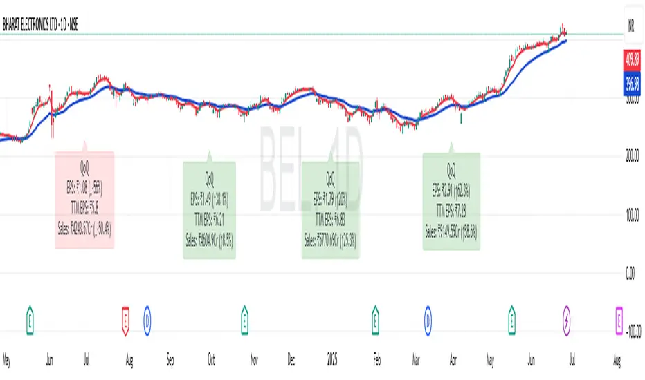
EPS and Sales Magic Indicator V2EPS and Sales Magic Indicator V2
EPS and Sales Magic Indicator V2
Short Title: EPS V2
Author: Trading_Tomm
Platform: TradingView (Pine Script v6)
License: Free for public use under fair usage guidelines
Overview
The EPS and Sales Magic Indicator V2 is a powerful stock fundamental visualization tool built specifically for TradingView users who wish to incorporate earnings intelligence directly onto their price chart. Designed and developed by Trading_Tomm, this upgraded version of the original 'EPS and Sales Magic Indicator' includes an enriched and more insightful presentation of company performance metrics — now with TTM EPS support, advanced color-coding, label sizing, and refined control options.
This indicator is tailored for retail traders, swing investors, and long-term fundamental analysts who need to view Quarter-over-Quarter (QoQ) earnings and revenue changes directly on the price chart without switching tabs or breaking focus.
What Does It Display?
The EPS and Sales Magic Indicator V2 intelligently detects quarterly financial updates and displays the following data points via labels:
1. EPS (Earnings Per Share) – Current Quarterly Value
This is the most recent Diluted EPS published by the company, fetched using TradingView’s request.financial() function.
Displayed in the format: EPS: ₹20.45
2. EPS QoQ Percentage Change
Shows the percentage change in EPS compared to the previous quarter.
Highlights improvement or decline using arrows (up for improvement, down for decline).
Displayed in the format: EPS: ₹20.45 (up 15.3 percent)
3. Sales (Revenue) – Current Quarterly Value
Fetches and displays Total Revenue of the company in ₹Crores for easier Indian-market readability.
Displayed in the format: Sales: ₹460Cr
4. Sales QoQ Percentage Change
Measures and presents the quarter-over-quarter percentage change in total revenue.
Uses arrows to indicate growth or contraction.
Displayed in the format: Sales: ₹460Cr (down 3.8 percent)
5. EPS TTM (Trailing Twelve Months)
You now get the TTM EPS — the sum of the last four quarterly EPS values.
This value provides a better long-term earnings snapshot compared to a single quarter.
Displayed in the format: TTM EPS: ₹78.12
All of these values are automatically calculated and displayed only on the bars where a new financial report is detected, keeping your chart clean and insightful.
Customization Features
This indicator is built with user control in mind, allowing you to personalize how and what you want to see:
Show EPS in Label: Enable or disable the display of EPS and EPS QoQ values.
Show Sales in Label: Toggle the visibility of revenue and sales change percentage.
Color Options for Label Themes: The label background color is automatically determined based on performance.
Green: Both EPS and Sales increased QoQ.
Red: Both decreased.
Orange: One increased and the other decreased.
Gray: Default color (if values are unavailable or mixed).
Label Text Size: Choose from Tiny, Small (default), or Normal.
Visual Design
Placement: The labels are positioned just below the candlesticks using yloc.belowbar, so they do not obstruct price action or interfere with technical indicators.
Anchor: Aligned precisely with the financial reporting bars to maintain clarity in historical comparisons.
Background Style: Clean, semi-transparent styling with soft text colors for comfortable viewing.
How It Works
The indicator relies on TradingView’s powerful request.financial() function to extract fiscal quarterly financials (FQ). Internally, it uses detection logic to identify fresh data updates by comparing current vs. previous values, arithmetic to compute QoQ percentage changes in EPS and Sales, logic to build formatted labels dynamically based on user selections, and conditional color and sizing logic to enhance interpretability.
Use Cases
For Long-Term Investors: Quickly identify if a company’s profitability and revenue are improving over time.
For Swing Traders: Combine recent earnings trends with price action to evaluate if post-result momentum has real backing.
For Technical and Fundamental Traders: Layer it with moving averages, RSI, or volume to create a hybrid analysis environment.
Limitations and Notes
Financial data is provided by TradingView’s financial API, and occasional missing values may occur for less-covered stocks.
This tool does not repaint but depends on the timing of the official financial updates.
All values are rounded and formatted to prioritize readability.
Works best on Daily or higher timeframes (weekly or monthly also supported).
License and Fair Use
This script is free to use and share under TradingView’s open-use guidelines. You may copy, fork, and build upon this indicator for personal or educational purposes, but commercial usage requires attribution to the author: Trading_Tomm.
Future Enhancements (Planned)
Addition of Net Profit (QoQ and TTM)
Inclusion of Operating Margin, Profit Margin, and Book Value
Option to switch between numeric and graphical display (table mode)
Alerts on extreme earnings deviation or sales slumps
Final Thoughts
The EPS and Sales Magic Indicator V2 represents a clean, visual, and smart way to monitor a company’s core performance from your chart screen. It helps you align fundamental strength with technical strategies and provides instant financial clarity, which is especially vital in today’s fast-moving markets.
Whether you’re preparing for an earnings season or scanning past performance to pick your next investment, this indicator saves time, enhances insights, and sharpens decisions.
The Sequences of FibonacciThe Sequences of Fibonacci - Advanced Multi-Timeframe Confluence Analysis System
THEORETICAL FOUNDATION & MATHEMATICAL INNOVATION
The Sequences of Fibonacci represents a revolutionary approach to market analysis that synthesizes classical Fibonacci mathematics with modern adaptive signal processing. This indicator transcends traditional Fibonacci retracement tools by implementing a sophisticated multi-dimensional confluence detection system that reveals hidden market structure through mathematical precision.
Core Mathematical Framework
Dynamic Fibonacci Grid System:
Unlike static Fibonacci tools, this system calculates highest highs and lowest lows across true Fibonacci sequence periods (8, 13, 21, 34, 55 bars) creating a dynamic grid of mathematical support and resistance levels that adapt to market structure in real-time.
Multi-Dimensional Confluence Detection:
The engine employs advanced mathematical clustering algorithms to identify areas where multiple derived Fibonacci retracement levels (0.382, 0.500, 0.618) from different timeframe perspectives converge. These "Confluence Zones" are mathematically classified by strength:
- CRITICAL Zones: 8+ converging Fibonacci levels
- HIGH Zones: 6-7 converging levels
- MEDIUM Zones: 4-5 converging levels
- LOW Zones: 3+ converging levels
Adaptive Signal Processing Architecture:
The system implements adaptive Stochastic RSI calculations with dynamic overbought/oversold levels that adjust to recent market volatility rather than using fixed thresholds. This prevents false signals during changing market conditions.
COMPREHENSIVE FEATURE ARCHITECTURE
Quantum Field Visualization System
Dynamic Price Field Mathematics:
The Quantum Field creates adaptive price channels based on EMA center points and ATR-based amplitude calculations, influenced by the Unified Field metric. This visualization system helps traders understand:
- Expected price volatility ranges
- Potential overextension zones
- Mathematical pressure points in market structure
- Dynamic support/resistance boundaries
Field Amplitude Calculation:
Field Amplitude = ATR × (1 + |Unified Field| / 10)
The system generates three quantum levels:
- Q⁰ Level: 0.618 × Field Amplitude (Primary channel)
- Q¹ Level: 1.0 × Field Amplitude (Secondary boundary)
- Q² Level: 1.618 × Field Amplitude (Extreme extension)
Advanced Market Analysis Dashboard
Unified Field Analysis:
A composite metric combining:
- Price momentum (40% weighting)
- Volume momentum (30% weighting)
- Trend strength (30% weighting)
Market Resonance Calculation:
Measures price-volume correlation over 14 periods to identify harmony between price action and volume participation.
Signal Quality Assessment:
Synthesizes Unified Field, Market Resonance, and RSI positioning to provide real-time evaluation of setup potential.
Tiered Signal Generation Logic
Tier 1 Signals (Highest Conviction):
Require ALL conditions:
- Adaptive StochRSI setup (exiting dynamic OB/OS levels)
- Classic StochRSI divergence confirmation
- Strong reversal bar pattern (adaptive ATR-based sizing)
- Level rejection from Confluence Zone or Fibonacci level
- Supportive Unified Field context
Tier 2 Signals (Enhanced Opportunity Detection):
Generated when Tier 1 conditions aren't met but exceptional circumstances exist:
- Divergence candidate patterns (relaxed divergence requirements)
- Exceptionally strong reversal bars at critical levels
- Enhanced level rejection criteria
- Maintained context filtering
Intelligent Visualization Features
Fractal Matrix Grid:
Multi-layer visualization system displaying:
- Shadow Layer: Foundational support (width 5)
- Glow Layer: Core identification (width 3, white)
- Quantum Layer: Mathematical overlay (width 1, dotted)
Smart Labeling System:
Prevents overlap using ATR-based minimum spacing while providing:
- Fibonacci period identification
- Topological complexity classification (0, I, II, III)
- Exact price levels
- Strength indicators (○ ◐ ● ⚡)
Wick Pressure Analysis:
Dynamic visualization showing momentum direction through:
- Multi-beam projection lines
- Particle density effects
- Progressive transparency for natural flow
- Strength-based sizing adaptation
PRACTICAL TRADING IMPLEMENTATION
Signal Interpretation Framework
Entry Protocol:
1. Confluence Zone Approach: Monitor price approaching High/Critical confluence zones
2. Adaptive Setup Confirmation: Wait for StochRSI to exit adaptive OB/OS levels
3. Divergence Verification: Confirm classic or candidate divergence patterns
4. Reversal Bar Assessment: Validate strong rejection using adaptive ATR criteria
5. Context Evaluation: Ensure Unified Field provides supportive environment
Risk Management Integration:
- Stop Placement: Beyond rejected confluence zone or Fibonacci level
- Position Sizing: Based on signal tier and confluence strength
- Profit Targets: Next significant confluence zone or quantum field boundary
Adaptive Parameter System
Dynamic StochRSI Levels:
Unlike fixed 80/20 levels, the system calculates adaptive OB/OS based on recent StochRSI range:
- Adaptive OB: Recent minimum + (range × OB percentile)
- Adaptive OS: Recent minimum + (range × OS percentile)
- Lookback Period: Configurable 20-100 bars for range calculation
Intelligent ATR Adaptation:
Bar size requirements adjust to market volatility:
- High Volatility: Reduced multiplier (bars naturally larger)
- Low Volatility: Increased multiplier (ensuring significance)
- Base Multiplier: 0.6× ATR with adaptive scaling
Optimization Guidelines
Timeframe-Specific Settings:
Scalping (1-5 minutes):
- Fibonacci Rejection Sensitivity: 0.3-0.8
- Confluence Threshold: 2-3 levels
- StochRSI Lookback: 20-30 bars
Day Trading (15min-1H):
- Fibonacci Rejection Sensitivity: 0.5-1.2
- Confluence Threshold: 3-4 levels
- StochRSI Lookback: 40-60 bars
Swing Trading (4H-1D):
- Fibonacci Rejection Sensitivity: 1.0-2.0
- Confluence Threshold: 4-5 levels
- StochRSI Lookback: 60-80 bars
Asset-Specific Optimization:
Cryptocurrency:
- Higher rejection sensitivity (1.0-2.5) for volatile conditions
- Enable Tier 2 signals for increased opportunity detection
- Shorter adaptive lookbacks for rapid market changes
Forex Major Pairs:
- Moderate sensitivity (0.8-1.5) for stable trending
- Focus on Higher/Critical confluence zones
- Longer lookbacks for institutional flow detection
Stock Indices:
- Conservative sensitivity (0.5-1.0) for institutional participation
- Standard confluence thresholds
- Balanced adaptive parameters
IMPORTANT USAGE CONSIDERATIONS
Realistic Performance Expectations
This indicator provides probabilistic advantages based on mathematical confluence analysis, not guaranteed outcomes. Signal quality varies with market conditions, and proper risk management remains essential regardless of signal tier.
Understanding Adaptive Features:
- Adaptive parameters react to historical data, not future market conditions
- Dynamic levels adjust to past volatility patterns
- Signal quality reflects mathematical alignment probability, not certainty
Market Context Awareness:
- Strong trending markets may produce fewer reversal signals
- Range-bound conditions typically generate more confluence opportunities
- News events and fundamental factors can override technical analysis
Educational Value
Mathematical Concepts Introduced:
- Multi-dimensional confluence analysis
- Adaptive signal processing techniques
- Dynamic parameter optimization
- Mathematical field theory applications in trading
- Advanced Fibonacci sequence applications
Skill Development Benefits:
- Understanding market structure through mathematical lens
- Recognition of multi-timeframe confluence principles
- Appreciation for adaptive vs. static analysis methods
- Integration of classical Fibonacci with modern signal processing
UNIQUE INNOVATIONS
First-Ever Implementations
1. True Fibonacci Sequence Periods: First indicator using authentic Fibonacci numbers (8,13,21,34,55) for timeframe analysis
2. Mathematical Confluence Clustering: Advanced algorithm identifying true Fibonacci level convergence
3. Adaptive StochRSI Boundaries: Dynamic OB/OS levels replacing fixed thresholds
4. Tiered Signal Architecture: Democratic signal weighting with quality classification
5. Quantum Field Price Visualization: Mathematical field representation of price dynamics
Visualization Breakthroughs
- Multi-Layer Fibonacci Grid: Three-layer rendering with intelligent spacing
- Dynamic Confluence Zones: Strength-based color coding and sizing
- Adaptive Parameter Display: Real-time visualization of dynamic calculations
- Mathematical Field Effects: Quantum-inspired price channel visualization
- Progressive Transparency Systems: Natural visual flow without chart clutter
COMPREHENSIVE DASHBOARD SYSTEM
Multi-Size Display Options
Small Dashboard: Core metrics for mobile/limited screen space
Normal Dashboard: Balanced information density for standard desktop use
Large Dashboard: Complete analysis suite including adaptive parameter values
Real-Time Metrics Tracking
Market Analysis Section:
- Unified Field strength with visual meter
- Market Resonance percentage
- Signal Quality assessment with emoji indicators
- Market Bias classification (Bullish/Bearish/Neutral)
Confluence Intelligence:
- Total active zones count
- High/Critical zone identification
- Nearest zone distance and strength
- Price-to-zone ATR measurement
Adaptive Parameters (Large Dashboard):
- Current StochRSI OB/OS levels
- Active ATR multiplier for bar sizing
- Volatility ratio for adaptive scaling
- Real-time StochRSI positioning
TECHNICAL SPECIFICATIONS
Pine Script Version: v5 (Latest)
Calculation Method: Real-time with confirmed bar processing
Maximum Objects: 500 boxes, 500 lines, 500 labels
Dashboard Positions: 4 corner options with size selection
Visual Themes: Quantum, Holographic, Crystalline, Plasma
Alert Integration: Complete alert system for all signal types
Performance Optimizations:
- Efficient confluence zone calculation using advanced clustering
- Smart label spacing prevents overlap
- Progressive transparency for visual clarity
- Memory-optimized array management
EDUCATIONAL FRAMEWORK
Learning Progression
Beginner Level:
- Understanding Fibonacci sequence applications
- Recognition of confluence zone concepts
- Basic signal interpretation
- Dashboard metric comprehension
Intermediate Level:
- Adaptive parameter optimization
- Multi-timeframe confluence analysis
- Signal quality assessment techniques
- Risk management integration
Advanced Level:
- Mathematical field theory applications
- Custom parameter optimization strategies
- Market regime adaptation techniques
- Professional trading system integration
DEVELOPMENT ACKNOWLEDGMENT
Special acknowledgment to @AlgoTrader90 - the foundational concepts of this system came from him and we developed it through a collaborative discussions about multi-timeframe Fibonacci analysis. While the original framework came from AlgoTrader90's innovative approach, this implementation represents a complete evolution of the logic with enhanced mathematical precision, adaptive parameters, and sophisticated signal filtering to deliver meaningful, actionable trading signals.
CONCLUSION
The Sequences of Fibonacci represents a quantum leap in technical analysis, successfully merging classical Fibonacci mathematics with cutting-edge adaptive signal processing. Through sophisticated confluence detection, intelligent parameter adaptation, and comprehensive market analysis, this system provides traders with unprecedented insight into market structure and potential reversal points.
The mathematical foundation ensures lasting relevance while the adaptive features maintain effectiveness across changing market conditions. From the dynamic Fibonacci grid to the quantum field visualization, every component reflects a commitment to mathematical precision, visual elegance, and practical utility.
Whether you're a beginner seeking to understand market confluence or an advanced trader requiring sophisticated analytical tools, this system provides the mathematical framework for informed decision-making based on time-tested Fibonacci principles enhanced with modern computational techniques.
Trade with mathematical precision. Trade with the power of confluence. Trade with The Sequences of Fibonacci.
"Mathematics is the language with which God has written the universe. In markets, Fibonacci sequences reveal the hidden harmonies that govern price movement, and those who understand these mathematical relationships hold the key to anticipating market behavior."
* Galileo Galilei (adapted for modern markets)
— Dskyz, Trade with insight. Trade with anticipation.

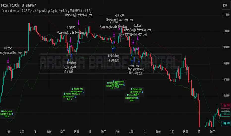
Quantum Reversal# 🧠 Quantum Reversal
## **Quantitative Mean Reversion Framework**
This algorithmic trading system employs **statistical mean reversion theory** combined with **adaptive volatility modeling** to capitalize on Bitcoin's inherent price oscillations around its statistical mean. The strategy integrates multiple technical indicators through a **multi-layered signal processing architecture**.
---
## ⚡ **Core Technical Architecture**
### 📊 **Statistical Foundation**
- **Bollinger Band Mean Reversion Model**: Utilizes 20-period moving average with 2.2 standard deviation bands for volatility-adjusted entry signals
- **Adaptive Volatility Threshold**: Dynamic standard deviation multiplier accounts for Bitcoin's heteroscedastic volatility patterns
- **Price Action Confluence**: Entry triggered when price breaches lower volatility band, indicating statistical oversold conditions
### 🔬 **Momentum Analysis Layer**
- **RSI Oscillator Integration**: 14-period Relative Strength Index with modified oversold threshold at 45
- **Signal Smoothing Algorithm**: 5-period simple moving average applied to RSI reduces noise and false signals
- **Momentum Divergence Detection**: Captures mean reversion opportunities when momentum indicators show oversold readings
### ⚙️ **Entry Logic Architecture**
```
Entry Condition = (Price ≤ Lower_BB) OR (Smoothed_RSI < 45)
```
- **Dual-Condition Framework**: Either statistical price deviation OR momentum oversold condition triggers entry
- **Boolean Logic Gate**: OR-based entry system increases signal frequency while maintaining statistical validity
- **Position Sizing**: Fixed 10% equity allocation per trade for consistent risk exposure
### 🎯 **Exit Strategy Optimization**
- **Profit-Lock Mechanism**: Positions only closed when showing positive unrealized P&L
- **Trend Continuation Logic**: Allows winning trades to run until momentum exhaustion
- **Dynamic Exit Timing**: No fixed profit targets - exits based on profitability state rather than arbitrary levels
---
## 📈 **Statistical Properties**
### **Risk Management Framework**
- **Long-Only Exposure**: Eliminates short-squeeze risk inherent in cryptocurrency markets
- **Mean Reversion Bias**: Exploits Bitcoin's tendency to revert to statistical mean after extreme moves
- **Position Management**: Single position limit prevents over-leveraging
### **Signal Processing Characteristics**
- **Noise Reduction**: SMA smoothing on RSI eliminates high-frequency oscillations
- **Volatility Adaptation**: Bollinger Bands automatically adjust to changing market volatility
- **Multi-Timeframe Coherence**: Indicators operate on consistent timeframe for signal alignment
---
## 🔧 **Parameter Configuration**
| Technical Parameter | Value | Statistical Significance |
|-------------------|-------|-------------------------|
| Bollinger Period | 20 | Standard statistical lookback for volatility calculation |
| Std Dev Multiplier | 2.2 | Optimized for Bitcoin's volatility distribution (95.4% confidence interval) |
| RSI Period | 14 | Traditional momentum oscillator period |
| RSI Threshold | 45 | Modified oversold level accounting for Bitcoin's momentum characteristics |
| Smoothing Period | 5 | Noise reduction filter for momentum signals |
---
## 📊 **Algorithmic Advantages**
✅ **Statistical Edge**: Exploits documented mean reversion tendency in Bitcoin markets
✅ **Volatility Adaptation**: Dynamic bands adjust to changing market conditions
✅ **Signal Confluence**: Multiple indicator confirmation reduces false positives
✅ **Momentum Integration**: RSI smoothing improves signal quality and timing
✅ **Risk-Controlled Exposure**: Systematic position sizing and long-only bias
---
## 🔬 **Mathematical Foundation**
The strategy leverages **Bollinger Band theory** (developed by John Bollinger) which assumes that prices tend to revert to the mean after extreme deviations. The RSI component adds **momentum confirmation** to the statistical price deviation signal.
**Statistical Basis:**
- Mean reversion follows the principle that extreme price deviations from the moving average are temporary
- The 2.2 standard deviation multiplier captures approximately 97.2% of price movements under normal distribution
- RSI momentum smoothing reduces noise inherent in oscillator calculations
---
## ⚠️ **Risk Considerations**
This algorithm is designed for traders with understanding of **quantitative finance principles** and **cryptocurrency market dynamics**. The strategy assumes mean-reverting behavior which may not persist during trending market phases. Proper risk management and position sizing are essential.
---
## 🎯 **Implementation Notes**
- **Market Regime Awareness**: Most effective in ranging/consolidating markets
- **Volatility Sensitivity**: Performance may vary during extreme volatility events
- **Backtesting Recommended**: Historical performance analysis advised before live implementation
- **Capital Allocation**: 10% per trade sizing assumes diversified portfolio approach
---
**Engineered for quantitative traders seeking systematic mean reversion exposure in Bitcoin markets through statistically-grounded technical analysis.**
Tensor Market Analysis Engine (TMAE)# Tensor Market Analysis Engine (TMAE)
## Advanced Multi-Dimensional Mathematical Analysis System
*Where Quantum Mathematics Meets Market Structure*
---
## 🎓 THEORETICAL FOUNDATION
The Tensor Market Analysis Engine represents a revolutionary synthesis of three cutting-edge mathematical frameworks that have never before been combined for comprehensive market analysis. This indicator transcends traditional technical analysis by implementing advanced mathematical concepts from quantum mechanics, information theory, and fractal geometry.
### 🌊 Multi-Dimensional Volatility with Jump Detection
**Hawkes Process Implementation:**
The TMAE employs a sophisticated Hawkes process approximation for detecting self-exciting market jumps. Unlike traditional volatility measures that treat price movements as independent events, the Hawkes process recognizes that market shocks cluster and exhibit memory effects.
**Mathematical Foundation:**
```
Intensity λ(t) = μ + Σ α(t - Tᵢ)
```
Where market jumps at times Tᵢ increase the probability of future jumps through the decay function α, controlled by the Hawkes Decay parameter (0.5-0.99).
**Mahalanobis Distance Calculation:**
The engine calculates volatility jumps using multi-dimensional Mahalanobis distance across up to 5 volatility dimensions:
- **Dimension 1:** Price volatility (standard deviation of returns)
- **Dimension 2:** Volume volatility (normalized volume fluctuations)
- **Dimension 3:** Range volatility (high-low spread variations)
- **Dimension 4:** Correlation volatility (price-volume relationship changes)
- **Dimension 5:** Microstructure volatility (intrabar positioning analysis)
This creates a volatility state vector that captures market behavior impossible to detect with traditional single-dimensional approaches.
### 📐 Hurst Exponent Regime Detection
**Fractal Market Hypothesis Integration:**
The TMAE implements advanced Rescaled Range (R/S) analysis to calculate the Hurst exponent in real-time, providing dynamic regime classification:
- **H > 0.6:** Trending (persistent) markets - momentum strategies optimal
- **H < 0.4:** Mean-reverting (anti-persistent) markets - contrarian strategies optimal
- **H ≈ 0.5:** Random walk markets - breakout strategies preferred
**Adaptive R/S Analysis:**
Unlike static implementations, the TMAE uses adaptive windowing that adjusts to market conditions:
```
H = log(R/S) / log(n)
```
Where R is the range of cumulative deviations and S is the standard deviation over period n.
**Dynamic Regime Classification:**
The system employs hysteresis to prevent regime flipping, requiring sustained Hurst values before regime changes are confirmed. This prevents false signals during transitional periods.
### 🔄 Transfer Entropy Analysis
**Information Flow Quantification:**
Transfer entropy measures the directional flow of information between price and volume, revealing lead-lag relationships that indicate future price movements:
```
TE(X→Y) = Σ p(yₜ₊₁, yₜ, xₜ) log
```
**Causality Detection:**
- **Volume → Price:** Indicates accumulation/distribution phases
- **Price → Volume:** Suggests retail participation or momentum chasing
- **Balanced Flow:** Market equilibrium or transition periods
The system analyzes multiple lag periods (2-20 bars) to capture both immediate and structural information flows.
---
## 🔧 COMPREHENSIVE INPUT SYSTEM
### Core Parameters Group
**Primary Analysis Window (10-100, Default: 50)**
The fundamental lookback period affecting all calculations. Optimization by timeframe:
- **1-5 minute charts:** 20-30 (rapid adaptation to micro-movements)
- **15 minute-1 hour:** 30-50 (balanced responsiveness and stability)
- **4 hour-daily:** 50-100 (smooth signals, reduced noise)
- **Asset-specific:** Cryptocurrency 20-35, Stocks 35-50, Forex 40-60
**Signal Sensitivity (0.1-2.0, Default: 0.7)**
Master control affecting all threshold calculations:
- **Conservative (0.3-0.6):** High-quality signals only, fewer false positives
- **Balanced (0.7-1.0):** Optimal risk-reward ratio for most trading styles
- **Aggressive (1.1-2.0):** Maximum signal frequency, requires careful filtering
**Signal Generation Mode:**
- **Aggressive:** Any component signals (highest frequency)
- **Confluence:** 2+ components agree (balanced approach)
- **Conservative:** All 3 components align (highest quality)
### Volatility Jump Detection Group
**Volatility Dimensions (2-5, Default: 3)**
Determines the mathematical space complexity:
- **2D:** Price + Volume volatility (suitable for clean markets)
- **3D:** + Range volatility (optimal for most conditions)
- **4D:** + Correlation volatility (advanced multi-asset analysis)
- **5D:** + Microstructure volatility (maximum sensitivity)
**Jump Detection Threshold (1.5-4.0σ, Default: 3.0σ)**
Standard deviations required for volatility jump classification:
- **Cryptocurrency:** 2.0-2.5σ (naturally volatile)
- **Stock Indices:** 2.5-3.0σ (moderate volatility)
- **Forex Major Pairs:** 3.0-3.5σ (typically stable)
- **Commodities:** 2.0-3.0σ (varies by commodity)
**Jump Clustering Decay (0.5-0.99, Default: 0.85)**
Hawkes process memory parameter:
- **0.5-0.7:** Fast decay (jumps treated as independent)
- **0.8-0.9:** Moderate clustering (realistic market behavior)
- **0.95-0.99:** Strong clustering (crisis/event-driven markets)
### Hurst Exponent Analysis Group
**Calculation Method Options:**
- **Classic R/S:** Original Rescaled Range (fast, simple)
- **Adaptive R/S:** Dynamic windowing (recommended for trading)
- **DFA:** Detrended Fluctuation Analysis (best for noisy data)
**Trending Threshold (0.55-0.8, Default: 0.60)**
Hurst value defining persistent market behavior:
- **0.55-0.60:** Weak trend persistence
- **0.65-0.70:** Clear trending behavior
- **0.75-0.80:** Strong momentum regimes
**Mean Reversion Threshold (0.2-0.45, Default: 0.40)**
Hurst value defining anti-persistent behavior:
- **0.35-0.45:** Weak mean reversion
- **0.25-0.35:** Clear ranging behavior
- **0.15-0.25:** Strong reversion tendency
### Transfer Entropy Parameters Group
**Information Flow Analysis:**
- **Price-Volume:** Classic flow analysis for accumulation/distribution
- **Price-Volatility:** Risk flow analysis for sentiment shifts
- **Multi-Timeframe:** Cross-timeframe causality detection
**Maximum Lag (2-20, Default: 5)**
Causality detection window:
- **2-5 bars:** Immediate causality (scalping)
- **5-10 bars:** Short-term flow (day trading)
- **10-20 bars:** Structural flow (swing trading)
**Significance Threshold (0.05-0.3, Default: 0.15)**
Minimum entropy for signal generation:
- **0.05-0.10:** Detect subtle information flows
- **0.10-0.20:** Clear causality only
- **0.20-0.30:** Very strong flows only
---
## 🎨 ADVANCED VISUAL SYSTEM
### Tensor Volatility Field Visualization
**Five-Layer Resonance Bands:**
The tensor field creates dynamic support/resistance zones that expand and contract based on mathematical field strength:
- **Core Layer (Purple):** Primary tensor field with highest intensity
- **Layer 2 (Neutral):** Secondary mathematical resonance
- **Layer 3 (Info Blue):** Tertiary harmonic frequencies
- **Layer 4 (Warning Gold):** Outer field boundaries
- **Layer 5 (Success Green):** Maximum field extension
**Field Strength Calculation:**
```
Field Strength = min(3.0, Mahalanobis Distance × Tensor Intensity)
```
The field amplitude adjusts to ATR and mathematical distance, creating dynamic zones that respond to market volatility.
**Radiation Line Network:**
During active tensor states, the system projects directional radiation lines showing field energy distribution:
- **8 Directional Rays:** Complete angular coverage
- **Tapering Segments:** Progressive transparency for natural visual flow
- **Pulse Effects:** Enhanced visualization during volatility jumps
### Dimensional Portal System
**Portal Mathematics:**
Dimensional portals visualize regime transitions using category theory principles:
- **Green Portals (◉):** Trending regime detection (appear below price for support)
- **Red Portals (◎):** Mean-reverting regime (appear above price for resistance)
- **Yellow Portals (○):** Random walk regime (neutral positioning)
**Tensor Trail Effects:**
Each portal generates 8 trailing particles showing mathematical momentum:
- **Large Particles (●):** Strong mathematical signal
- **Medium Particles (◦):** Moderate signal strength
- **Small Particles (·):** Weak signal continuation
- **Micro Particles (˙):** Signal dissipation
### Information Flow Streams
**Particle Stream Visualization:**
Transfer entropy creates flowing particle streams indicating information direction:
- **Upward Streams:** Volume leading price (accumulation phases)
- **Downward Streams:** Price leading volume (distribution phases)
- **Stream Density:** Proportional to information flow strength
**15-Particle Evolution:**
Each stream contains 15 particles with progressive sizing and transparency, creating natural flow visualization that makes information transfer immediately apparent.
### Fractal Matrix Grid System
**Multi-Timeframe Fractal Levels:**
The system calculates and displays fractal highs/lows across five Fibonacci periods:
- **8-Period:** Short-term fractal structure
- **13-Period:** Intermediate-term patterns
- **21-Period:** Primary swing levels
- **34-Period:** Major structural levels
- **55-Period:** Long-term fractal boundaries
**Triple-Layer Visualization:**
Each fractal level uses three-layer rendering:
- **Shadow Layer:** Widest, darkest foundation (width 5)
- **Glow Layer:** Medium white core line (width 3)
- **Tensor Layer:** Dotted mathematical overlay (width 1)
**Intelligent Labeling System:**
Smart spacing prevents label overlap using ATR-based minimum distances. Labels include:
- **Fractal Period:** Time-based identification
- **Topological Class:** Mathematical complexity rating (0, I, II, III)
- **Price Level:** Exact fractal price
- **Mahalanobis Distance:** Current mathematical field strength
- **Hurst Exponent:** Current regime classification
- **Anomaly Indicators:** Visual strength representations (○ ◐ ● ⚡)
### Wick Pressure Analysis
**Rejection Level Mathematics:**
The system analyzes candle wick patterns to project future pressure zones:
- **Upper Wick Analysis:** Identifies selling pressure and resistance zones
- **Lower Wick Analysis:** Identifies buying pressure and support zones
- **Pressure Projection:** Extends lines forward based on mathematical probability
**Multi-Layer Glow Effects:**
Wick pressure lines use progressive transparency (1-8 layers) creating natural glow effects that make pressure zones immediately visible without cluttering the chart.
### Enhanced Regime Background
**Dynamic Intensity Mapping:**
Background colors reflect mathematical regime strength:
- **Deep Transparency (98% alpha):** Subtle regime indication
- **Pulse Intensity:** Based on regime strength calculation
- **Color Coding:** Green (trending), Red (mean-reverting), Neutral (random)
**Smoothing Integration:**
Regime changes incorporate 10-bar smoothing to prevent background flicker while maintaining responsiveness to genuine regime shifts.
### Color Scheme System
**Six Professional Themes:**
- **Dark (Default):** Professional trading environment optimization
- **Light:** High ambient light conditions
- **Classic:** Traditional technical analysis appearance
- **Neon:** High-contrast visibility for active trading
- **Neutral:** Minimal distraction focus
- **Bright:** Maximum visibility for complex setups
Each theme maintains mathematical accuracy while optimizing visual clarity for different trading environments and personal preferences.
---
## 📊 INSTITUTIONAL-GRADE DASHBOARD
### Tensor Field Status Section
**Field Strength Display:**
Real-time Mahalanobis distance calculation with dynamic emoji indicators:
- **⚡ (Lightning):** Extreme field strength (>1.5× threshold)
- **● (Solid Circle):** Strong field activity (>1.0× threshold)
- **○ (Open Circle):** Normal field state
**Signal Quality Rating:**
Democratic algorithm assessment:
- **ELITE:** All 3 components aligned (highest probability)
- **STRONG:** 2 components aligned (good probability)
- **GOOD:** 1 component active (moderate probability)
- **WEAK:** No clear component signals
**Threshold and Anomaly Monitoring:**
- **Threshold Display:** Current mathematical threshold setting
- **Anomaly Level (0-100%):** Combined volatility and volume spike measurement
- **>70%:** High anomaly (red warning)
- **30-70%:** Moderate anomaly (orange caution)
- **<30%:** Normal conditions (green confirmation)
### Tensor State Analysis Section
**Mathematical State Classification:**
- **↑ BULL (Tensor State +1):** Trending regime with bullish bias
- **↓ BEAR (Tensor State -1):** Mean-reverting regime with bearish bias
- **◈ SUPER (Tensor State 0):** Random walk regime (neutral)
**Visual State Gauge:**
Five-circle progression showing tensor field polarity:
- **🟢🟢🟢⚪⚪:** Strong bullish mathematical alignment
- **⚪⚪🟡⚪⚪:** Neutral/transitional state
- **⚪⚪🔴🔴🔴:** Strong bearish mathematical alignment
**Trend Direction and Phase Analysis:**
- **📈 BULL / 📉 BEAR / ➡️ NEUTRAL:** Primary trend classification
- **🌪️ CHAOS:** Extreme information flow (>2.0 flow strength)
- **⚡ ACTIVE:** Strong information flow (1.0-2.0 flow strength)
- **😴 CALM:** Low information flow (<1.0 flow strength)
### Trading Signals Section
**Real-Time Signal Status:**
- **🟢 ACTIVE / ⚪ INACTIVE:** Long signal availability
- **🔴 ACTIVE / ⚪ INACTIVE:** Short signal availability
- **Components (X/3):** Active algorithmic components
- **Mode Display:** Current signal generation mode
**Signal Strength Visualization:**
Color-coded component count:
- **Green:** 3/3 components (maximum confidence)
- **Aqua:** 2/3 components (good confidence)
- **Orange:** 1/3 components (moderate confidence)
- **Gray:** 0/3 components (no signals)
### Performance Metrics Section
**Win Rate Monitoring:**
Estimated win rates based on signal quality with emoji indicators:
- **🔥 (Fire):** ≥60% estimated win rate
- **👍 (Thumbs Up):** 45-59% estimated win rate
- **⚠️ (Warning):** <45% estimated win rate
**Mathematical Metrics:**
- **Hurst Exponent:** Real-time fractal dimension (0.000-1.000)
- **Information Flow:** Volume/price leading indicators
- **📊 VOL:** Volume leading price (accumulation/distribution)
- **💰 PRICE:** Price leading volume (momentum/speculation)
- **➖ NONE:** Balanced information flow
- **Volatility Classification:**
- **🔥 HIGH:** Above 1.5× jump threshold
- **📊 NORM:** Normal volatility range
- **😴 LOW:** Below 0.5× jump threshold
### Market Structure Section (Large Dashboard)
**Regime Classification:**
- **📈 TREND:** Hurst >0.6, momentum strategies optimal
- **🔄 REVERT:** Hurst <0.4, contrarian strategies optimal
- **🎲 RANDOM:** Hurst ≈0.5, breakout strategies preferred
**Mathematical Field Analysis:**
- **Dimensions:** Current volatility space complexity (2D-5D)
- **Hawkes λ (Lambda):** Self-exciting jump intensity (0.00-1.00)
- **Jump Status:** 🚨 JUMP (active) / ✅ NORM (normal)
### Settings Summary Section (Large Dashboard)
**Active Configuration Display:**
- **Sensitivity:** Current master sensitivity setting
- **Lookback:** Primary analysis window
- **Theme:** Active color scheme
- **Method:** Hurst calculation method (Classic R/S, Adaptive R/S, DFA)
**Dashboard Sizing Options:**
- **Small:** Essential metrics only (mobile/small screens)
- **Normal:** Balanced information density (standard desktop)
- **Large:** Maximum detail (multi-monitor setups)
**Position Options:**
- **Top Right:** Standard placement (avoids price action)
- **Top Left:** Wide chart optimization
- **Bottom Right:** Recent price focus (scalping)
- **Bottom Left:** Maximum price visibility (swing trading)
---
## 🎯 SIGNAL GENERATION LOGIC
### Multi-Component Convergence System
**Component Signal Architecture:**
The TMAE generates signals through sophisticated component analysis rather than simple threshold crossing:
**Volatility Component:**
- **Jump Detection:** Mahalanobis distance threshold breach
- **Hawkes Intensity:** Self-exciting process activation (>0.2)
- **Multi-dimensional:** Considers all volatility dimensions simultaneously
**Hurst Regime Component:**
- **Trending Markets:** Price above SMA-20 with positive momentum
- **Mean-Reverting Markets:** Price at Bollinger Band extremes
- **Random Markets:** Bollinger squeeze breakouts with directional confirmation
**Transfer Entropy Component:**
- **Volume Leadership:** Information flow from volume to price
- **Volume Spike:** Volume 110%+ above 20-period average
- **Flow Significance:** Above entropy threshold with directional bias
### Democratic Signal Weighting
**Signal Mode Implementation:**
- **Aggressive Mode:** Any single component triggers signal
- **Confluence Mode:** Minimum 2 components must agree
- **Conservative Mode:** All 3 components must align
**Momentum Confirmation:**
All signals require momentum confirmation:
- **Long Signals:** RSI >50 AND price >EMA-9
- **Short Signals:** RSI <50 AND price 0.6):**
- **Increase Sensitivity:** Catch momentum continuation
- **Lower Mean Reversion Threshold:** Avoid counter-trend signals
- **Emphasize Volume Leadership:** Institutional accumulation/distribution
- **Tensor Field Focus:** Use expansion for trend continuation
- **Signal Mode:** Aggressive or Confluence for trend following
**Range-Bound Markets (Hurst <0.4):**
- **Decrease Sensitivity:** Avoid false breakouts
- **Lower Trending Threshold:** Quick regime recognition
- **Focus on Price Leadership:** Retail sentiment extremes
- **Fractal Grid Emphasis:** Support/resistance trading
- **Signal Mode:** Conservative for high-probability reversals
**Volatile Markets (High Jump Frequency):**
- **Increase Hawkes Decay:** Recognize event clustering
- **Higher Jump Threshold:** Avoid noise signals
- **Maximum Dimensions:** Capture full volatility complexity
- **Reduce Position Sizing:** Risk management adaptation
- **Enhanced Visuals:** Maximum information for rapid decisions
**Low Volatility Markets (Low Jump Frequency):**
- **Decrease Jump Threshold:** Capture subtle movements
- **Lower Hawkes Decay:** Treat moves as independent
- **Reduce Dimensions:** Simplify analysis
- **Increase Position Sizing:** Capitalize on compressed volatility
- **Minimal Visuals:** Reduce distraction in quiet markets
---
## 🚀 ADVANCED TRADING STRATEGIES
### The Mathematical Convergence Method
**Entry Protocol:**
1. **Fractal Grid Approach:** Monitor price approaching significant fractal levels
2. **Tensor Field Confirmation:** Verify field expansion supporting direction
3. **Portal Signal:** Wait for dimensional portal appearance
4. **ELITE/STRONG Quality:** Only trade highest quality mathematical signals
5. **Component Consensus:** Confirm 2+ components agree in Confluence mode
**Example Implementation:**
- Price approaching 21-period fractal high
- Tensor field expanding upward (bullish mathematical alignment)
- Green portal appears below price (trending regime confirmation)
- ELITE quality signal with 3/3 components active
- Enter long position with stop below fractal level
**Risk Management:**
- **Stop Placement:** Below/above fractal level that generated signal
- **Position Sizing:** Based on Mahalanobis distance (higher distance = smaller size)
- **Profit Targets:** Next fractal level or tensor field resistance
### The Regime Transition Strategy
**Regime Change Detection:**
1. **Monitor Hurst Exponent:** Watch for persistent moves above/below thresholds
2. **Portal Color Change:** Regime transitions show different portal colors
3. **Background Intensity:** Increasing regime background intensity
4. **Mathematical Confirmation:** Wait for regime confirmation (hysteresis)
**Trading Implementation:**
- **Trending Transitions:** Trade momentum breakouts, follow trend
- **Mean Reversion Transitions:** Trade range boundaries, fade extremes
- **Random Transitions:** Trade breakouts with tight stops
**Advanced Techniques:**
- **Multi-Timeframe:** Confirm regime on higher timeframe
- **Early Entry:** Enter on regime transition rather than confirmation
- **Regime Strength:** Larger positions during strong regime signals
### The Information Flow Momentum Strategy
**Flow Detection Protocol:**
1. **Monitor Transfer Entropy:** Watch for significant information flow shifts
2. **Volume Leadership:** Strong edge when volume leads price
3. **Flow Acceleration:** Increasing flow strength indicates momentum
4. **Directional Confirmation:** Ensure flow aligns with intended trade direction
**Entry Signals:**
- **Volume → Price Flow:** Enter during accumulation/distribution phases
- **Price → Volume Flow:** Enter on momentum confirmation breaks
- **Flow Reversal:** Counter-trend entries when flow reverses
**Optimization:**
- **Scalping:** Use immediate flow detection (2-5 bar lag)
- **Swing Trading:** Use structural flow (10-20 bar lag)
- **Multi-Asset:** Compare flow between correlated assets
### The Tensor Field Expansion Strategy
**Field Mathematics:**
The tensor field expansion indicates mathematical pressure building in market structure:
**Expansion Phases:**
1. **Compression:** Field contracts, volatility decreases
2. **Tension Building:** Mathematical pressure accumulates
3. **Expansion:** Field expands rapidly with directional movement
4. **Resolution:** Field stabilizes at new equilibrium
**Trading Applications:**
- **Compression Trading:** Prepare for breakout during field contraction
- **Expansion Following:** Trade direction of field expansion
- **Reversion Trading:** Fade extreme field expansion
- **Multi-Dimensional:** Consider all field layers for confirmation
### The Hawkes Process Event Strategy
**Self-Exciting Jump Trading:**
Understanding that market shocks cluster and create follow-on opportunities:
**Jump Sequence Analysis:**
1. **Initial Jump:** First volatility jump detected
2. **Clustering Phase:** Hawkes intensity remains elevated
3. **Follow-On Opportunities:** Additional jumps more likely
4. **Decay Period:** Intensity gradually decreases
**Implementation:**
- **Jump Confirmation:** Wait for mathematical jump confirmation
- **Direction Assessment:** Use other components for direction
- **Clustering Trades:** Trade subsequent moves during high intensity
- **Decay Exit:** Exit positions as Hawkes intensity decays
### The Fractal Confluence System
**Multi-Timeframe Fractal Analysis:**
Combining fractal levels across different periods for high-probability zones:
**Confluence Zones:**
- **Double Confluence:** 2 fractal levels align
- **Triple Confluence:** 3+ fractal levels cluster
- **Mathematical Confirmation:** Tensor field supports the level
- **Information Flow:** Transfer entropy confirms direction
**Trading Protocol:**
1. **Identify Confluence:** Find 2+ fractal levels within 1 ATR
2. **Mathematical Support:** Verify tensor field alignment
3. **Signal Quality:** Wait for STRONG or ELITE signal
4. **Risk Definition:** Use fractal level for stop placement
5. **Profit Targeting:** Next major fractal confluence zone
---
## ⚠️ COMPREHENSIVE RISK MANAGEMENT
### Mathematical Position Sizing
**Mahalanobis Distance Integration:**
Position size should inversely correlate with mathematical field strength:
```
Position Size = Base Size × (Threshold / Mahalanobis Distance)
```
**Risk Scaling Matrix:**
- **Low Field Strength (<2.0):** Standard position sizing
- **Moderate Field Strength (2.0-3.0):** 75% position sizing
- **High Field Strength (3.0-4.0):** 50% position sizing
- **Extreme Field Strength (>4.0):** 25% position sizing or no trade
### Signal Quality Risk Adjustment
**Quality-Based Position Sizing:**
- **ELITE Signals:** 100% of planned position size
- **STRONG Signals:** 75% of planned position size
- **GOOD Signals:** 50% of planned position size
- **WEAK Signals:** No position or paper trading only
**Component Agreement Scaling:**
- **3/3 Components:** Full position size
- **2/3 Components:** 75% position size
- **1/3 Components:** 50% position size or skip trade
### Regime-Adaptive Risk Management
**Trending Market Risk:**
- **Wider Stops:** Allow for trend continuation
- **Trend Following:** Trade with regime direction
- **Higher Position Size:** Trend probability advantage
- **Momentum Stops:** Trail stops based on momentum indicators
**Mean-Reverting Market Risk:**
- **Tighter Stops:** Quick exits on trend continuation
- **Contrarian Positioning:** Trade against extremes
- **Smaller Position Size:** Higher reversal failure rate
- **Level-Based Stops:** Use fractal levels for stops
**Random Market Risk:**
- **Breakout Focus:** Trade only clear breakouts
- **Tight Initial Stops:** Quick exit if breakout fails
- **Reduced Frequency:** Skip marginal setups
- **Range-Based Targets:** Profit targets at range boundaries
### Volatility-Adaptive Risk Controls
**High Volatility Periods:**
- **Reduced Position Size:** Account for wider price swings
- **Wider Stops:** Avoid noise-based exits
- **Lower Frequency:** Skip marginal setups
- **Faster Exits:** Take profits more quickly
**Low Volatility Periods:**
- **Standard Position Size:** Normal risk parameters
- **Tighter Stops:** Take advantage of compressed ranges
- **Higher Frequency:** Trade more setups
- **Extended Targets:** Allow for compressed volatility expansion
### Multi-Timeframe Risk Alignment
**Higher Timeframe Trend:**
- **With Trend:** Standard or increased position size
- **Against Trend:** Reduced position size or skip
- **Neutral Trend:** Standard position size with tight management
**Risk Hierarchy:**
1. **Primary:** Current timeframe signal quality
2. **Secondary:** Higher timeframe trend alignment
3. **Tertiary:** Mathematical field strength
4. **Quaternary:** Market regime classification
---
## 📚 EDUCATIONAL VALUE AND MATHEMATICAL CONCEPTS
### Advanced Mathematical Concepts
**Tensor Analysis in Markets:**
The TMAE introduces traders to tensor analysis, a branch of mathematics typically reserved for physics and advanced engineering. Tensors provide a framework for understanding multi-dimensional market relationships that scalar and vector analysis cannot capture.
**Information Theory Applications:**
Transfer entropy implementation teaches traders about information flow in markets, a concept from information theory that quantifies directional causality between variables. This provides intuition about market microstructure and participant behavior.
**Fractal Geometry in Trading:**
The Hurst exponent calculation exposes traders to fractal geometry concepts, helping understand that markets exhibit self-similar patterns across multiple timeframes. This mathematical insight transforms how traders view market structure.
**Stochastic Process Theory:**
The Hawkes process implementation introduces concepts from stochastic process theory, specifically self-exciting point processes. This provides mathematical framework for understanding why market events cluster and exhibit memory effects.
### Learning Progressive Complexity
**Beginner Mathematical Concepts:**
- **Volatility Dimensions:** Understanding multi-dimensional analysis
- **Regime Classification:** Learning market personality types
- **Signal Democracy:** Algorithmic consensus building
- **Visual Mathematics:** Interpreting mathematical concepts visually
**Intermediate Mathematical Applications:**
- **Mahalanobis Distance:** Statistical distance in multi-dimensional space
- **Rescaled Range Analysis:** Fractal dimension measurement
- **Information Entropy:** Quantifying uncertainty and causality
- **Field Theory:** Understanding mathematical fields in market context
**Advanced Mathematical Integration:**
- **Tensor Field Dynamics:** Multi-dimensional market force analysis
- **Stochastic Self-Excitation:** Event clustering and memory effects
- **Categorical Composition:** Mathematical signal combination theory
- **Topological Market Analysis:** Understanding market shape and connectivity
### Practical Mathematical Intuition
**Developing Market Mathematics Intuition:**
The TMAE serves as a bridge between abstract mathematical concepts and practical trading applications. Traders develop intuitive understanding of:
- **How markets exhibit mathematical structure beneath apparent randomness**
- **Why multi-dimensional analysis reveals patterns invisible to single-variable approaches**
- **How information flows through markets in measurable, predictable ways**
- **Why mathematical models provide probabilistic edges rather than certainties**
---
## 🔬 IMPLEMENTATION AND OPTIMIZATION
### Getting Started Protocol
**Phase 1: Observation (Week 1)**
1. **Apply with defaults:** Use standard settings on your primary trading timeframe
2. **Study visual elements:** Learn to interpret tensor fields, portals, and streams
3. **Monitor dashboard:** Observe how metrics change with market conditions
4. **No trading:** Focus entirely on pattern recognition and understanding
**Phase 2: Pattern Recognition (Week 2-3)**
1. **Identify signal patterns:** Note what market conditions produce different signal qualities
2. **Regime correlation:** Observe how Hurst regimes affect signal performance
3. **Visual confirmation:** Learn to read tensor field expansion and portal signals
4. **Component analysis:** Understand which components drive signals in different markets
**Phase 3: Parameter Optimization (Week 4-5)**
1. **Asset-specific tuning:** Adjust parameters for your specific trading instrument
2. **Timeframe optimization:** Fine-tune for your preferred trading timeframe
3. **Sensitivity adjustment:** Balance signal frequency with quality
4. **Visual customization:** Optimize colors and intensity for your trading environment
**Phase 4: Live Implementation (Week 6+)**
1. **Paper trading:** Test signals with hypothetical trades
2. **Small position sizing:** Begin with minimal risk during learning phase
3. **Performance tracking:** Monitor actual vs. expected signal performance
4. **Continuous optimization:** Refine settings based on real performance data
### Performance Monitoring System
**Signal Quality Tracking:**
- **ELITE Signal Win Rate:** Track highest quality signals separately
- **Component Performance:** Monitor which components provide best signals
- **Regime Performance:** Analyze performance across different market regimes
- **Timeframe Analysis:** Compare performance across different session times
**Mathematical Metric Correlation:**
- **Field Strength vs. Performance:** Higher field strength should correlate with better performance
- **Component Agreement vs. Win Rate:** More component agreement should improve win rates
- **Regime Alignment vs. Success:** Trading with mathematical regime should outperform
### Continuous Optimization Process
**Monthly Review Protocol:**
1. **Performance Analysis:** Review win rates, profit factors, and maximum drawdown
2. **Parameter Assessment:** Evaluate if current settings remain optimal
3. **Market Adaptation:** Adjust for changes in market character or volatility
4. **Component Weighting:** Consider if certain components should receive more/less emphasis
**Quarterly Deep Analysis:**
1. **Mathematical Model Validation:** Verify that mathematical relationships remain valid
2. **Regime Distribution:** Analyze time spent in different market regimes
3. **Signal Evolution:** Track how signal characteristics change over time
4. **Correlation Analysis:** Monitor correlations between different mathematical components
---
## 🌟 UNIQUE INNOVATIONS AND CONTRIBUTIONS
### Revolutionary Mathematical Integration
**First-Ever Implementations:**
1. **Multi-Dimensional Volatility Tensor:** First indicator to implement true tensor analysis for market volatility
2. **Real-Time Hawkes Process:** First trading implementation of self-exciting point processes
3. **Transfer Entropy Trading Signals:** First practical application of information theory for trade generation
4. **Democratic Component Voting:** First algorithmic consensus system for signal generation
5. **Fractal-Projected Signal Quality:** First system to predict signal quality at future price levels
### Advanced Visualization Innovations
**Mathematical Visualization Breakthroughs:**
- **Tensor Field Radiation:** Visual representation of mathematical field energy
- **Dimensional Portal System:** Category theory visualization for regime transitions
- **Information Flow Streams:** Real-time visual display of market information transfer
- **Multi-Layer Fractal Grid:** Intelligent spacing and projection system
- **Regime Intensity Mapping:** Dynamic background showing mathematical regime strength
### Practical Trading Innovations
**Trading System Advances:**
- **Quality-Weighted Signal Generation:** Signals rated by mathematical confidence
- **Regime-Adaptive Strategy Selection:** Automatic strategy optimization based on market personality
- **Anti-Spam Signal Protection:** Mathematical prevention of signal clustering
- **Component Performance Tracking:** Real-time monitoring of algorithmic component success
- **Field-Strength Position Sizing:** Mathematical volatility integration for risk management
---
## ⚖️ RESPONSIBLE USAGE AND LIMITATIONS
### Mathematical Model Limitations
**Understanding Model Boundaries:**
While the TMAE implements sophisticated mathematical concepts, traders must understand fundamental limitations:
- **Markets Are Not Purely Mathematical:** Human psychology, news events, and fundamental factors create unpredictable elements
- **Past Performance Limitations:** Mathematical relationships that worked historically may not persist indefinitely
- **Model Risk:** Complex models can fail during unprecedented market conditions
- **Overfitting Potential:** Highly optimized parameters may not generalize to future market conditions
### Proper Implementation Guidelines
**Risk Management Requirements:**
- **Never Risk More Than 2% Per Trade:** Regardless of signal quality
- **Diversification Mandatory:** Don't rely solely on mathematical signals
- **Position Sizing Discipline:** Use mathematical field strength for sizing, not confidence
- **Stop Loss Non-Negotiable:** Every trade must have predefined risk parameters
**Realistic Expectations:**
- **Mathematical Edge, Not Certainty:** The indicator provides probabilistic advantages, not guaranteed outcomes
- **Learning Curve Required:** Complex mathematical concepts require time to master
- **Market Adaptation Necessary:** Parameters must evolve with changing market conditions
- **Continuous Education Important:** Understanding underlying mathematics improves application
### Ethical Trading Considerations
**Market Impact Awareness:**
- **Information Asymmetry:** Advanced mathematical analysis may provide advantages over other market participants
- **Position Size Responsibility:** Large positions based on mathematical signals can impact market structure
- **Sharing Knowledge:** Consider educational contributions to trading community
- **Fair Market Participation:** Use mathematical advantages responsibly within market framework
### Professional Development Path
**Skill Development Sequence:**
1. **Basic Mathematical Literacy:** Understand fundamental concepts before advanced application
2. **Risk Management Mastery:** Develop disciplined risk control before relying on complex signals
3. **Market Psychology Understanding:** Combine mathematical analysis with behavioral market insights
4. **Continuous Learning:** Stay updated on mathematical finance developments and market evolution
---
## 🔮 CONCLUSION
The Tensor Market Analysis Engine represents a quantum leap forward in technical analysis, successfully bridging the gap between advanced pure mathematics and practical trading applications. By integrating multi-dimensional volatility analysis, fractal market theory, and information flow dynamics, the TMAE reveals market structure invisible to conventional analysis while maintaining visual clarity and practical usability.
### Mathematical Innovation Legacy
This indicator establishes new paradigms in technical analysis:
- **Tensor analysis for market volatility understanding**
- **Stochastic self-excitation for event clustering prediction**
- **Information theory for causality-based trade generation**
- **Democratic algorithmic consensus for signal quality enhancement**
- **Mathematical field visualization for intuitive market understanding**
### Practical Trading Revolution
Beyond mathematical innovation, the TMAE transforms practical trading:
- **Quality-rated signals replace binary buy/sell decisions**
- **Regime-adaptive strategies automatically optimize for market personality**
- **Multi-dimensional risk management integrates mathematical volatility measures**
- **Visual mathematical concepts make complex analysis immediately interpretable**
- **Educational value creates lasting improvement in trading understanding**
### Future-Proof Design
The mathematical foundations ensure lasting relevance:
- **Universal mathematical principles transcend market evolution**
- **Multi-dimensional analysis adapts to new market structures**
- **Regime detection automatically adjusts to changing market personalities**
- **Component democracy allows for future algorithmic additions**
- **Mathematical visualization scales with increasing market complexity**
### Commitment to Excellence
The TMAE represents more than an indicator—it embodies a philosophy of bringing rigorous mathematical analysis to trading while maintaining practical utility and visual elegance. Every component, from the multi-dimensional tensor fields to the democratic signal generation, reflects a commitment to mathematical accuracy, trading practicality, and educational value.
### Trading with Mathematical Precision
In an era where markets grow increasingly complex and computational, the TMAE provides traders with mathematical tools previously available only to institutional quantitative research teams. Yet unlike academic mathematical models, the TMAE translates complex concepts into intuitive visual representations and practical trading signals.
By combining the mathematical rigor of tensor analysis, the statistical power of multi-dimensional volatility modeling, and the information-theoretic insights of transfer entropy, traders gain unprecedented insight into market structure and dynamics.
### Final Perspective
Markets, like nature, exhibit profound mathematical beauty beneath apparent chaos. The Tensor Market Analysis Engine serves as a mathematical lens that reveals this hidden order, transforming how traders perceive and interact with market structure.
Through mathematical precision, visual elegance, and practical utility, the TMAE empowers traders to see beyond the noise and trade with the confidence that comes from understanding the mathematical principles governing market behavior.
Trade with mathematical insight. Trade with the power of tensors. Trade with the TMAE.
*"In mathematics, you don't understand things. You just get used to them." - John von Neumann*
*With the TMAE, mathematical market understanding becomes not just possible, but intuitive.*
— Dskyz, Trade with insight. Trade with anticipation.

RMSE Bollinger Bands + Loop | Lyro RSRMSE Bollinger Bands + Loops
Overview
The RMSE Bollinger Bands + Loops is a sophisticated technical analysis tool designed to identify and quantify market trends by combining dynamic moving averages with statistical measures. This indicator employs a multi-model approach, integrating Bollinger-style RMSE bands, momentum scoring, and a hybrid signal system to provide traders with adaptive insights across varying market conditions.
Indicator Modes
Bollinger-style RMSE Bands: this mode calculates dynamic volatility bands around the price using the following formula:
Upper Band = Dynamic Moving Average + (RMSE × Multiplier)
Lower Band = Dynamic Moving Average - (RMSE × Multiplier)
These bands adjust to market volatility, helping identify potential breakout or breakdown points.
For-Loop Momentum Scoring, momentum is assessed by analyzing recent price behavior through a looping mechanism. A rising momentum score indicates increasing bullish strength, while a declining score suggests growing bearish momentum.
Hybrid Combined Signal: this mode assigns a directional score to the other two modes:
+1 for bullish (green)
–1 for bearish (red)
An average of these scores is computed to generate a combined signal, offering a consolidated market trend indication.
Practical Application
Signal Interpretation: A buy signal is generated when both the RMSE Bands and For-Loop Momentum Scoring align bullishly. Conversely, a sell signal is indicated when both are bearish.
Trend Confirmation: The Hybrid Combined Signal provides a consolidated view, assisting traders in confirming the prevailing market trend.
Note: Always consider additional technical analysis tools and risk management strategies when making trading decisions.
⚠️Disclaimer
This indicator is a tool for technical analysis and does not provide guaranteed results. It should be used in conjunction with other analysis methods and proper risk management practices. The creators of this indicator are not responsible for any financial decisions made based on its signals.
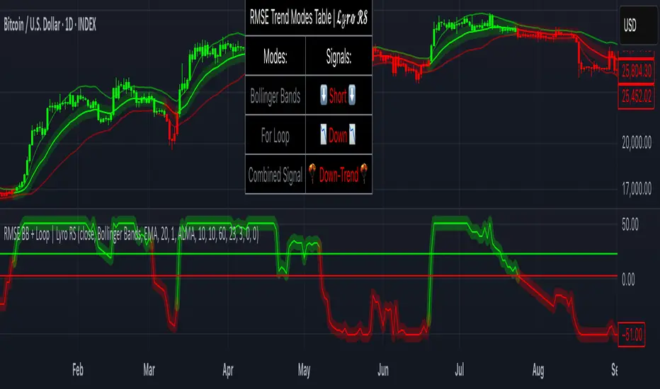
Data Monitoring TableThis is a visual data dashboard specifically designed for users engaged in quantitative trading and technical analysis. It is equipped with two data tables that can dynamically display key market technical indicators and cryptocurrency price fluctuation data, supporting customizable column configurations and trading mode filtering.
✅ Core Features:
Intuitive display of critical technical indicators, including the Relative Strength Index (RSI), K-line entity gain, upper/lower shadow ratio, trading volume level, and change rate.
Multi-timeframe tracking of price fluctuations for BTC/ETH/SOL/XRP/DOGE (1-day, 6-hour, 3-hour).
Selectable trading modes: "long-only", "short-only", or "both".
Customizable number of columns to adapt to analysis needs across different timeframes.
All data is visualized in tables with color-coded prompts for market conditions (overbought, oversold, high volatility, low volatility, etc.).
📈 Target Audience:
Investors seeking systematic access to technical data.
Quantitative strategy developers aiming to capture market structural changes.
Intermediate and beginner traders looking to enhance market intuition and decision-making.
New Feature:
We have added a trading volume monitoring grade setting feature. Users can set the monitoring grade by themselves. When the market trading volume reaches this grade, the system will trigger an alarm. The default setting is level 5. This setting is designed to filter out trades with small fluctuations, helping users to capture key trading signals more accurately and improve the efficiency of trading decisions.
中文介绍
这是一款专为量化交易和技术分析用户设计的可视化数据仪表盘。它配备两个数据表格,可动态展示关键市场技术指标与加密货币价格波动数据,支持自定义列配置和交易模式筛选。
✅ 核心功能:
直观展示相对强弱指标(RSI)、K 线实体涨幅、上下影线比例、成交量水平及变化率等关键技术指标。
多时间框架追踪 BTC/ETH/SOL/XRP/DOGE 价格波动(1 日、6 小时、3 小时)。
可选交易模式:“仅做多”“仅做空” 或 “多空双向”。
可自定义列数,适配不同时间框架的分析需求。
所有数据以表格可视化呈现,通过颜色标注提示市场状况(超买、超卖、高波动、低波动等)。
📈 目标用户:
寻求系统获取技术数据的投资者。
旨在捕捉市场结构变化的量化策略开发者。
希望提升市场洞察力和决策能力的初、中级交易者。
新增功能:
我们新增了成交量监控等级设置功能。用户可自行设定监控等级,当市场成交量达到该等级时,系统将触发警报。默认设置为 5 级,此设置旨在过滤掉小幅波动的交易,帮助用户更精准地捕捉关键交易信号,提升交易决策效率。

SOT & SA Detector ProSOT & SA Detector Pro- Advanced Reversal Pattern Recognition
OVERVIEW
The SOT & SA Detector is an educational indicator designed to identify potential market reversal points through systematic analysis of candlestick patterns, volume confirmation, and price wave structures. SOT (Shorting of Thrust) signals suggest potential bearish reversals after upward price movements, while SA (Selling Accumulation) signals indicate possible bullish reversals following downward trends. This tool helps traders recognize key market transition points by combining multiple technical criteria for enhanced signal reliability.
═══════════════════════════════════════════════════════════════
HOW IT WORKS
Technical Methodology
The indicator employs a multi-factor analysis approach that evaluates:
Wave Structure Analysis: Identifies minimum 2-bar directional waves (upward for SOT, downward for SA)
Price Delta Validation: Ensures closing price changes remain within specified percentage thresholds (default 0.3%) best 0.1.
Candlestick Tail Analysis: Measures rejection wicks using configurable tail multipliers
Volume Confirmation: Requires increased volume compared to previous periods
Pattern Confirmation: Validates signals through subsequent price action
Signal Generation Process
Pattern Recognition: Scans for qualifying candlestick formations with appropriate tail characteristics
Volume Verification: Confirms patterns with volume expansion using adjustable multiplier
Price Confirmation: Validates signals when price breaks and closes beyond pattern extremes
Signal Display: Places labeled markers and draws horizontal reference levels
Mathematical Foundation
Delta calculation: math.abs(close - close ) / close <= deltaPercent / 100
Tail analysis: (high - close ) >= tailMultiplier * (close - low ) for SOT
Volume filter: volume >= volume * volumeFactor
═══════════════════════════════════════════════════════════════
KEY FEATURES
Dual Pattern Recognition: Identifies both bullish (SA) and bearish (SOT) reversal candidates
Volume Integration: Incorporates volume analysis for enhanced signal validation
Customizable Parameters: Adjustable wave length, delta percentage, tail multiplier, and volume factor
Visual Clarity: Color-coded bar highlighting, labeled signals, and horizontal reference levels
Time-Based Filtering: Configurable analysis period to focus on recent market activity
Non-Repainting Signals: Confirmed signals remain stable and do not change with new price data
Alert System: Built-in notifications for both initial signals and subsequent confirmations
═══════════════════════════════════════════════════════════════
HOW TO USE
Signal Interpretation
Red SOT Labels: Appear above potential bearish reversal candles with downward-pointing markers
Green SA Labels: Display below potential bullish reversal candles with upward-pointing markers
Horizontal Lines: Extend from signal levels to provide ongoing reference points
Bar Coloring: Highlights qualifying pattern candles for visual emphasis
Trading Application
This indicator serves as an educational tool for pattern recognition and should be used in conjunction with additional analysis methods. Consider SOT signals as potential areas of selling pressure following upward moves, while SA signals may indicate buying interest after downward price action.
Best Practices
Combine with trend analysis and support/resistance levels
Consider overall market context and timeframe alignment
Use proper risk management techniques
Validate signals with additional technical indicators
═══════════════════════════════════════════════════════════════
SETTINGS
Analysis Days (Default: 20)
Controls the lookback period for signal detection. Higher values extend historical analysis while lower values focus on recent activity.
Minimum Bars in Wave (Default: 2)
Sets the minimum consecutive bars required to establish directional wave patterns. Increase for stronger trend confirmation.
Max Close Change % (Default: 0.3) best 0.1.
Defines acceptable closing price variation between consecutive bars. Lower values require tighter price consolidation.
Tail Multiplier (Default: 1.0) best 1.5 or more.
Adjusts sensitivity for candlestick tail analysis. Higher values require more pronounced rejection wicks.
Volume Factor (Default: 1.0)
Sets volume expansion threshold compared to previous period. Values above 1.0 require volume increases.
═══════════════════════════════════════════════════════════════
LIMITATIONS
Market Conditions
May produce false signals in highly volatile or low-volume conditions
Effectiveness varies across different market environments and timeframes
Requires sufficient volume data for optimal performance
Signal Timing
Signals appear after pattern completion, not in real-time during formation
Confirmation signals depend on subsequent price action
Historical signals do not guarantee future market behavior
Technical Constraints
Limited to analyzing price and volume data only
Does not incorporate fundamental analysis or external market factors
Performance may vary significantly across different trading instruments
═══════════════════════════════════════════════════════════════
IMPORTANT DISCLAIMERS
This indicator is designed for educational purposes and technical analysis learning. It does not constitute financial advice, investment recommendations, or trading signals. Past performance does not guarantee future results. Trading involves substantial risk of loss, and this tool should be used alongside proper risk management techniques and additional analysis methods.
Always conduct thorough analysis using multiple indicators and consider market context before making trading decisions. The SOT & SA patterns represent potential reversal points but do not guarantee price direction changes.
═══════════════════════════════════════════════════════════════
Credits: Original concept and Pine Script implementation by Everyday_Trader_X
Version: Pine Script v6 compatible
Category: Technical Analysis / Reversal Detection
Overlay: Yes (displays on price chart)
Volatility Quality [Alpha Extract]The Alpha-Extract Volatility Quality (AVQ) Indicator provides traders with deep insights into market volatility by measuring the directional strength of price movements. This sophisticated momentum-based tool helps identify overbought and oversold conditions, offering actionable buy and sell signals based on volatility trends and standard deviation bands.
🔶 CALCULATION
The indicator processes volatility quality data through a series of analytical steps:
Bar Range Calculation: Measures true range (TR) to capture price volatility.
Directional Weighting: Applies directional bias (positive for bullish candles, negative for bearish) to the true range.
VQI Computation: Uses an exponential moving average (EMA) of weighted volatility to derive the Volatility Quality Index (VQI).
vqiRaw = ta.ema(weightedVol, vqiLen)
Smoothing: Applies an additional EMA to smooth the VQI for clearer signals.
Normalization: Optionally normalizes VQI to a -100/+100 scale based on historical highs and lows.
Standard Deviation Bands: Calculates three upper and lower bands using standard deviation multipliers for volatility thresholds.
vqiStdev = ta.stdev(vqiSmoothed, vqiLen)
upperBand1 = vqiSmoothed + (vqiStdev * stdevMultiplier1)
upperBand2 = vqiSmoothed + (vqiStdev * stdevMultiplier2)
upperBand3 = vqiSmoothed + (vqiStdev * stdevMultiplier3)
lowerBand1 = vqiSmoothed - (vqiStdev * stdevMultiplier1)
lowerBand2 = vqiSmoothed - (vqiStdev * stdevMultiplier2)
lowerBand3 = vqiSmoothed - (vqiStdev * stdevMultiplier3)
Signal Generation: Produces overbought/oversold signals when VQI reaches extreme levels (±200 in normalized mode).
Formula:
Bar Range = True Range (TR)
Weighted Volatility = Bar Range × (Close > Open ? 1 : Close < Open ? -1 : 0)
VQI Raw = EMA(Weighted Volatility, VQI Length)
VQI Smoothed = EMA(VQI Raw, Smoothing Length)
VQI Normalized = ((VQI Smoothed - Lowest VQI) / (Highest VQI - Lowest VQI) - 0.5) × 200
Upper Band N = VQI Smoothed + (StdDev(VQI Smoothed, VQI Length) × Multiplier N)
Lower Band N = VQI Smoothed - (StdDev(VQI Smoothed, VQI Length) × Multiplier N)
🔶 DETAILS
Visual Features:
VQI Plot: Displays VQI as a line or histogram (lime for positive, red for negative).
Standard Deviation Bands: Plots three upper and lower bands (teal for upper, grayscale for lower) to indicate volatility thresholds.
Reference Levels: Horizontal lines at 0 (neutral), +100, and -100 (in normalized mode) for context.
Zone Highlighting: Overbought (⋎ above bars) and oversold (⋏ below bars) signals for extreme VQI levels (±200 in normalized mode).
Candle Coloring: Optional candle overlay colored by VQI direction (lime for positive, red for negative).
Interpretation:
VQI ≥ 200 (Normalized): Overbought condition, strong sell signal.
VQI 100–200: High volatility, potential selling opportunity.
VQI 0–100: Neutral bullish momentum.
VQI 0 to -100: Neutral bearish momentum.
VQI -100 to -200: High volatility, strong bearish momentum.
VQI ≤ -200 (Normalized): Oversold condition, strong buy signal.
🔶 EXAMPLES
Overbought Signal Detection: When VQI exceeds 200 (normalized), the indicator flags potential market tops with a red ⋎ symbol.
Example: During strong uptrends, VQI reaching 200 has historically preceded corrections, allowing traders to secure profits.
Oversold Signal Detection: When VQI falls below -200 (normalized), a lime ⋏ symbol highlights potential buying opportunities.
Example: In bearish markets, VQI dropping below -200 has marked reversal points for profitable long entries.
Volatility Trend Tracking: The VQI plot and bands help traders visualize shifts in market momentum.
Example: A rising VQI crossing above zero with widening bands indicates strengthening bullish momentum, guiding traders to hold or enter long positions.
Dynamic Support/Resistance: Standard deviation bands act as dynamic volatility thresholds during price movements.
Example: Price reversals often occur near the third standard deviation bands, providing reliable entry/exit points during volatile periods.
🔶 SETTINGS
Customization Options:
VQI Length: Adjust the EMA period for VQI calculation (default: 14, range: 1–50).
Smoothing Length: Set the EMA period for smoothing (default: 5, range: 1–50).
Standard Deviation Multipliers: Customize multipliers for bands (defaults: 1.0, 2.0, 3.0).
Normalization: Toggle normalization to -100/+100 scale and adjust lookback period (default: 200, min: 50).
Display Style: Switch between line or histogram plot for VQI.
Candle Overlay: Enable/disable VQI-colored candles (lime for positive, red for negative).
The Alpha-Extract Volatility Quality Indicator empowers traders with a robust tool to navigate market volatility. By combining directional price range analysis with smoothed volatility metrics, it identifies overbought and oversold conditions, offering clear buy and sell signals. The customizable standard deviation bands and optional normalization provide precise context for market conditions, enabling traders to make informed decisions across various market cycles.
Multifractal Forecast [ScorsoneEnterprises]Multifractal Forecast Indicator
The Multifractal Forecast is an indicator designed to model and forecast asset price movements using a multifractal framework. It uses concepts from fractal geometry and stochastic processes, specifically the Multifractal Model of Asset Returns (MMAR) and fractional Brownian motion (fBm), to generate price forecasts based on historical price data. The indicator visualizes potential future price paths as colored lines, providing traders with a probabilistic view of price trends over a specified trading time scale. Below is a detailed breakdown of the indicator’s functionality, inputs, calculations, and visualization.
Overview
Purpose: The indicator forecasts future price movements by simulating multiple price paths based on a multifractal model, which accounts for the complex, non-linear behavior of financial markets.
Key Concepts:
Multifractal Model of Asset Returns (MMAR): Models price movements as a multifractal process, capturing varying degrees of volatility and self-similarity across different time scales.
Fractional Brownian Motion (fBm): A generalization of Brownian motion that incorporates long-range dependence and self-similarity, controlled by the Hurst exponent.
Binomial Cascade: Used to model trading time, introducing heterogeneity in time scales to reflect market activity bursts.
Hurst Exponent: Measures the degree of long-term memory in the price series (persistence, randomness, or mean-reversion).
Rescaled Range (R/S) Analysis: Estimates the Hurst exponent to quantify the fractal nature of the price series.
Inputs
The indicator allows users to customize its behavior through several input parameters, each influencing the multifractal model and forecast generation:
Maximum Lag (max_lag):
Type: Integer
Default: 50
Minimum: 5
Purpose: Determines the maximum lag used in the rescaled range (R/S) analysis to calculate the Hurst exponent. A higher lag increases the sample size for Hurst estimation but may smooth out short-term dynamics.
2 to the n values in the Multifractal Model (n):
Type: Integer
Default: 4
Purpose: Defines the resolution of the multifractal model by setting the size of arrays used in calculations (N = 2^n). For example, n=4 results in N=16 data points. Larger n increases computational complexity and detail but may exceed Pine Script’s array size limits (capped at 100,000).
Multiplier for Binomial Cascade (m):
Type: Float
Default: 0.8
Purpose: Controls the asymmetry in the binomial cascade, which models trading time. The multiplier m (and its complement 2.0 - m) determines how mass is distributed across time scales. Values closer to 1 create more balanced cascades, while values further from 1 introduce more variability.
Length Scale for fBm (L):
Type: Float
Default: 100,000.0
Purpose: Scales the fractional Brownian motion output, affecting the amplitude of simulated price paths. Larger values increase the magnitude of forecasted price movements.
Cumulative Sum (cum):
Type: Integer (0 or 1)
Default: 1
Purpose: Toggles whether the fBm output is cumulatively summed (1=On, 0=Off). When enabled, the fBm series is accumulated to simulate a price path with memory, resembling a random walk with long-range dependence.
Trading Time Scale (T):
Type: Integer
Default: 5
Purpose: Defines the forecast horizon in bars (20 bars into the future). It also scales the binomial cascade’s output to align with the desired trading time frame.
Number of Simulations (num_simulations):
Type: Integer
Default: 5
Minimum: 1
Purpose: Specifies how many forecast paths are simulated and plotted. More simulations provide a broader range of possible price outcomes but increase computational load.
Core Calculations
The indicator combines several mathematical and statistical techniques to generate price forecasts. Below is a step-by-step explanation of its calculations:
Log Returns (lgr):
The indicator calculates log returns as math.log(close / close ) when both the current and previous close prices are positive. This measures the relative price change in a logarithmic scale, which is standard for financial time series analysis to stabilize variance.
Hurst Exponent Estimation (get_hurst_exponent):
Purpose: Estimates the Hurst exponent (H) to quantify the degree of long-term memory in the price series.
Method: Uses rescaled range (R/S) analysis:
For each lag from 2 to max_lag, the function calc_rescaled_range computes the rescaled range:
Calculate the mean of the log returns over the lag period.
Compute the cumulative deviation from the mean.
Find the range (max - min) of the cumulative deviation.
Divide the range by the standard deviation of the log returns to get the rescaled range.
The log of the rescaled range (log(R/S)) is regressed against the log of the lag (log(lag)) using the polyfit_slope function.
The slope of this regression is the Hurst exponent (H).
Interpretation:
H = 0.5: Random walk (no memory, like standard Brownian motion).
H > 0.5: Persistent behavior (trends tend to continue).
H < 0.5: Mean-reverting behavior (price tends to revert to the mean).
Fractional Brownian Motion (get_fbm):
Purpose: Generates a fractional Brownian motion series to model price movements with long-range dependence.
Inputs: n (array size 2^n), H (Hurst exponent), L (length scale), cum (cumulative sum toggle).
Method:
Computes covariance for fBm using the formula: 0.5 * (|i+1|^(2H) - 2 * |i|^(2H) + |i-1|^(2H)).
Uses Hosking’s method (referenced from Columbia University’s implementation) to generate fBm:
Initializes arrays for covariance (cov), intermediate calculations (phi, psi), and output.
Iteratively computes the fBm series by incorporating a random term scaled by the variance (v) and covariance structure.
Applies scaling based on L / N^H to adjust the amplitude.
Optionally applies cumulative summation if cum = 1 to produce a path with memory.
Output: An array of 2^n values representing the fBm series.
Binomial Cascade (get_binomial_cascade):
Purpose: Models trading time (theta) to account for non-uniform market activity (e.g., bursts of volatility).
Inputs: n (array size 2^n), m (multiplier), T (trading time scale).
Method:
Initializes an array of size 2^n with values of 1.0.
Iteratively applies a binomial cascade:
For each block (from 0 to n-1), splits the array into segments.
Randomly assigns a multiplier (m or 2.0 - m) to each segment, redistributing mass.
Normalizes the array by dividing by its sum and scales by T.
Checks for array size limits to prevent Pine Script errors.
Output: An array (theta) representing the trading time, which warps the fBm to reflect market activity.
Interpolation (interpolate_fbm):
Purpose: Maps the fBm series to the trading time scale to produce a forecast.
Method:
Computes the cumulative sum of theta and normalizes it to .
Interpolates the fBm series linearly based on the normalized trading time.
Ensures the output aligns with the trading time scale (T).
Output: An array of interpolated fBm values representing log returns over the forecast horizon.
Price Path Generation:
For each simulation (up to num_simulations):
Generates an fBm series using get_fbm.
Interpolates it with the trading time (theta) using interpolate_fbm.
Converts log returns to price levels:
Starts with the current close price.
For each step i in the forecast horizon (T), computes the price as prev_price * exp(log_return).
Output: An array of price levels for each simulation.
Visualization:
Trigger: Updates every T bars when the bar state is confirmed (barstate.isconfirmed).
Process:
Clears previous lines from line_array.
For each simulation, plots a line from the current bar’s close price to the forecasted price at bar_index + T.
Colors the line using a gradient (color.from_gradient) based on the final forecasted price relative to the minimum and maximum forecasted prices across all simulations (red for lower prices, teal for higher prices).
Output: Multiple colored lines on the chart, each representing a possible price path over the next T bars.
How It Works on the Chart
Initialization: On each bar, the indicator calculates the Hurst exponent (H) using historical log returns and prepares the trading time (theta) using the binomial cascade.
Forecast Generation: Every T bars, it generates num_simulations price paths:
Each path starts at the current close price.
Uses fBm to model log returns, warped by the trading time.
Converts log returns to price levels.
Plotting: Draws lines from the current bar to the forecasted price T bars ahead, with colors indicating relative price levels.
Dynamic Updates: The forecast updates every T bars, replacing old lines with new ones based on the latest price data and calculations.
Key Features
Multifractal Modeling: Captures complex market dynamics by combining fBm (long-range dependence) with a binomial cascade (non-uniform time).
Customizable Parameters: Allows users to adjust the forecast horizon, model resolution, scaling, and number of simulations.
Probabilistic Forecast: Multiple simulations provide a range of possible price outcomes, helping traders assess uncertainty.
Visual Clarity: Gradient-colored lines make it easy to distinguish bullish (teal) and bearish (red) forecasts.
Potential Use Cases
Trend Analysis: Identify potential price trends or reversals based on the direction and spread of forecast lines.
Risk Assessment: Evaluate the range of possible price outcomes to gauge market uncertainty.
Volatility Analysis: The Hurst exponent and binomial cascade provide insights into market persistence and volatility clustering.
Limitations
Computational Intensity: Large values of n or num_simulations may slow down execution or hit Pine Script’s array size limits.
Randomness: The binomial cascade and fBm rely on random terms (math.random), which may lead to variability between runs.
Assumptions: The model assumes log-normal price movements and fractal behavior, which may not always hold in extreme market conditions.
Adjusting Inputs:
Set max_lag based on the desired depth of historical analysis.
Adjust n for model resolution (start with 4–6 to avoid performance issues).
Tune m to control trading time variability (0.5–1.5 is typical).
Set L to scale the forecast amplitude (experiment with values like 10,000–1,000,000).
Choose T based on your trading horizon (20 for short-term, 50 for longer-term for example).
Select num_simulations for the number of forecast paths (5–10 is reasonable for visualization).
Interpret Output:
Teal lines suggest bullish scenarios, red lines suggest bearish scenarios.
A wide spread of lines indicates high uncertainty; convergence suggests a stronger trend.
Monitor Updates: Forecasts update every T bars, so check the chart periodically for new projections.
Chart Examples
This is a daily AMEX:SPY chart with default settings. We see the simulations being done every T bars and they provide a range for us to analyze with a few simulations still in the range.
On this intraday PEPPERSTONE:COCOA chart I modified the Length Scale for fBm, L, parameter to be 1000 from 100000. Adjusting the parameter as you switch between timeframes can give you more contextual simulations.
On BITSTAMP:ETHUSD I modified the L to be 1000000 to have a more contextual set of simulations with crypto's volatile nature.
With L at 100000 we see the range for NASDAQ:TLT is correctly simulated. The recent pop stays within the bounds of the highest simulation. Note this is a cherry picked example to show the power and potential of these simulations.
Technical Notes
Error Handling: The script includes checks for array size limits and division by zero (math.abs(denominator) > 1e-10, v := math.max(v, 1e-10)).
External Reference: The fBm implementation is based on Hosking’s method (www.columbia.edu), ensuring a robust algorithm.
Conclusion
The Multifractal Forecast is a powerful tool for traders seeking to model complex market dynamics using a multifractal framework. By combining fBm, binomial cascades, and Hurst exponent analysis, it generates probabilistic price forecasts that account for long-range dependence and non-uniform market activity. Its customizable inputs and clear visualizations make it suitable for both technical analysis and strategy development, though users should be mindful of its computational demands and parameter sensitivity. For optimal use, experiment with input settings and validate forecasts against other technical indicators or market conditions.
Fibonacci Entry Bands [AlgoAlpha]OVERVIEW
This script plots Fibonacci Entry Bands, a trend-following and mean-reversion hybrid system built around dynamic volatility-adjusted bands scaled using key Fibonacci levels. It calculates a smoothed basis line and overlays multiple bands at fixed Fibonacci multipliers of either ATR or standard deviation. Depending on the trend direction, specific upper or lower bands become active, offering a clear framework for entry timing, trend identification, and profit-taking zones.
CONCEPTS
The core idea is to use Fibonacci levels—0.618, 1.0, 1.618, and 2.618—as multipliers on a volatility measure to form layered price bands around a trend-following moving average. Trends are defined by whether the basis is rising or falling. The trend determines which side of the bands is emphasized: upper bands for downtrends, lower bands for uptrends. This approach captures both directional bias and extreme price extensions. Take-profit logic is built in via crossovers relative to the outermost bands, scaled by user-selected aggressiveness.
FEATURES
Basis Line – A double EMA smoothing of the source defines trend direction and acts as the central mean.
Volatility Bands – Four levels per side (based on selected ATR or stdev) mark the Fibonacci bands. These become visible only when trend direction matches the side (e.g., only lower bands plot in an uptrend).
Bar Coloring – Bars are shaded with adjustable transparency depending on distance from the basis, with color intensity helping gauge overextension.
Entry Arrows – A trend shift triggers either a long or short signal, with a marker at the outermost band with ▲/▼ signs.
Take-Profit Crosses – If price rejects near the outer band (based on aggressiveness setting), a cross appears marking potential profit-taking.
Bounce Signals – Minor pullbacks that respect the basis line are marked with triangle arrows, hinting at continuation setups.
Customization – Users can toggle bar coloring, signal markers, and select between ATR/stdev as well as take-profit aggressiveness.
Alerts – All major signals, including entries, take-profits, and bounces, are available as alert conditions.
USAGE
To use this tool, load it on your chart, adjust the inputs for volatility method and aggressiveness, and wait for entries to form on trend changes. Use TP crosses and bounce arrows as potential exit or scale-in signals.

Magnificent 7 OscillatorThe Magnificent 7 Oscillator is a sophisticated momentum-based technical indicator designed to analyze the collective performance of the seven largest technology companies in the U.S. stock market (Apple, Microsoft, Alphabet, Amazon, NVIDIA, Tesla, and Meta). This indicator incorporates established momentum factor research and provides three distinct analytical modes: absolute momentum tracking, equal-weighted market comparison, and relative performance analysis. The tool integrates five different oscillator methodologies and includes advanced breadth analysis capabilities.
Theoretical Foundation
Momentum Factor Research
The indicator's foundation rests on seminal momentum research in financial markets. Jegadeesh and Titman (1993) demonstrated that stocks with strong price performance over 3-12 month periods tend to continue outperforming in subsequent periods¹. This momentum effect was later incorporated into formal factor models by Carhart (1997), who extended the Fama-French three-factor model to include a momentum factor (UMD - Up Minus Down)².
The momentum calculation methodology follows the academic standard:
Momentum(t) = / P(t-n) × 100
Where P(t) is the current price and n is the lookback period.
The focus on the "Magnificent 7" stocks reflects the increasing market concentration observed in recent years. Fama and French (2015) noted that a small number of large-cap stocks can drive significant market movements due to their substantial index weights³. The combined market capitalization of these seven companies often exceeds 25% of the total S&P 500, making their collective momentum a critical market indicator.
Indicator Architecture
Core Components
1. Data Collection and Processing
The indicator employs robust data collection with error handling for missing or invalid security data. Each stock's momentum is calculated independently using the specified lookback period (default: 14 periods).
2. Composite Oscillator Calculation
Following Fama-French factor construction methodology, the indicator offers two weighting schemes:
- Equal Weight: Each active stock receives identical weighting (1/n)
- Market Cap Weight: Reserved for future enhancement
3. Oscillator Transformation Functions
The indicator provides five distinct oscillator types, each with established technical analysis foundations:
a) Momentum Oscillator (Default)
- Pure rate-of-change calculation
- Centered around zero
- Direct implementation of Jegadeesh & Titman methodology
b) RSI (Relative Strength Index)
- Wilder's (1978) relative strength methodology
- Transformed to center around zero for consistency
- Scale: -50 to +50
c) Stochastic Oscillator
- George Lane's %K methodology
- Measures current position within recent range
- Transformed to center around zero
d) Williams %R
- Larry Williams' range-based oscillator
- Inverse stochastic calculation
- Adjusted for zero-centered display
e) CCI (Commodity Channel Index)
- Donald Lambert's mean reversion indicator
- Measures deviation from moving average
- Scaled for optimal visualization
Operational Modes
Mode 1: Magnificent 7 Analysis
Tracks the collective momentum of the seven constituent stocks. This mode is optimal for:
- Technology sector analysis
- Growth stock momentum assessment
- Large-cap performance tracking
Mode 2: S&P 500 Equal Weight Comparison
Analyzes momentum using an equal-weighted S&P 500 reference (typically RSP ETF). This mode provides:
- Broader market momentum context
- Size-neutral market analysis
- Comparison baseline for relative performance
Mode 3: Relative Performance Analysis
Calculates the momentum differential between Magnificent 7 and S&P 500 Equal Weight. This mode enables:
- Sector rotation analysis
- Style factor assessment (Growth vs. Value)
- Relative strength identification
Formula: Relative Performance = MAG7_Momentum - SP500EW_Momentum
Signal Generation and Thresholds
Signal Classification
The indicator generates three signal states:
- Bullish: Oscillator > Upper Threshold (default: +2.0%)
- Bearish: Oscillator < Lower Threshold (default: -2.0%)
- Neutral: Oscillator between thresholds
Relative Performance Signals
In relative performance mode, specialized thresholds apply:
- Outperformance: Relative momentum > +1.0%
- Underperformance: Relative momentum < -1.0%
Alert System
Comprehensive alert conditions include:
- Threshold crossovers (bullish/bearish signals)
- Zero-line crosses (momentum direction changes)
- Relative performance shifts
- Breadth Analysis Component
The indicator incorporates market breadth analysis, calculating the percentage of constituent stocks with positive momentum. This feature provides insights into:
- Strong Breadth (>60%): Broad-based momentum
- Weak Breadth (<40%): Narrow momentum leadership
- Mixed Breadth (40-60%): Neutral momentum distribution
Visual Design and User Interface
Theme-Adaptive Display
The indicator automatically adjusts color schemes for dark and light chart themes, ensuring optimal visibility across different user preferences.
Professional Data Table
A comprehensive data table displays:
- Current oscillator value and percentage
- Active mode and oscillator type
- Signal status and strength
- Component breakdowns (in relative performance mode)
- Breadth percentage
- Active threshold levels
Custom Color Options
Users can override default colors with custom selections for:
- Neutral conditions (default: Material Blue)
- Bullish signals (default: Material Green)
- Bearish signals (default: Material Red)
Practical Applications
Portfolio Management
- Sector Allocation: Use relative performance mode to time technology sector exposure
- Risk Management: Monitor breadth deterioration as early warning signal
- Entry/Exit Timing: Utilize threshold crossovers for position sizing decisions
Market Analysis
- Trend Identification: Zero-line crosses indicate momentum regime changes
- Divergence Analysis: Compare MAG7 performance against broader market
- Volatility Assessment: Oscillator range and frequency provide volatility insights
Strategy Development
- Factor Timing: Implement growth factor timing strategies
- Momentum Strategies: Develop systematic momentum-based approaches
- Risk Parity: Use breadth metrics for risk-adjusted portfolio construction
Configuration Guidelines
Parameter Selection
- Momentum Period (5-100): Shorter periods (5-20) for tactical analysis, longer periods (50-100) for strategic assessment
- Smoothing Period (1-50): Higher values reduce noise but increase lag
- Thresholds: Adjust based on historical volatility and strategy requirements
Timeframe Considerations
- Daily Charts: Optimal for swing trading and medium-term analysis
- Weekly Charts: Suitable for long-term trend analysis
- Intraday Charts: Useful for short-term tactical decisions
Limitations and Considerations
Market Concentration Risk
The indicator's focus on seven stocks creates concentration risk. During periods of significant rotation away from large-cap technology stocks, the indicator may not represent broader market conditions.
Momentum Persistence
While momentum effects are well-documented, they are not permanent. Jegadeesh and Titman (1993) noted momentum reversal effects over longer time horizons (2-5 years).
Correlation Dynamics
During market stress, correlations among the constituent stocks may increase, reducing the diversification benefits and potentially amplifying signal intensity.
Performance Metrics and Backtesting
The indicator includes hidden plots for comprehensive backtesting:
- Individual stock momentum values
- Composite breadth percentage
- S&P 500 Equal Weight momentum
- Relative performance calculations
These metrics enable quantitative strategy development and historical performance analysis.
References
¹Jegadeesh, N., & Titman, S. (1993). Returns to buying winners and selling losers: Implications for stock market efficiency. Journal of Finance, 48(1), 65-91.
Carhart, M. M. (1997). On persistence in mutual fund performance. Journal of Finance, 52(1), 57-82.
Fama, E. F., & French, K. R. (2015). A five-factor asset pricing model. Journal of Financial Economics, 116(1), 1-22.
Wilder, J. W. (1978). New concepts in technical trading systems. Trend Research.
Multi TF Oscillators Screener [TradingFinder] RSI / ATR / Stoch🔵 Introduction
The oscillator screener is designed to simplify multi-timeframe analysis by allowing traders and analysts to monitor one or multiple symbols across their preferred timeframes—all at the same time. Users can track a single symbol through various timeframes simultaneously or follow multiple symbols in selected intervals. This flexibility makes the tool highly effective for analyzing diverse markets concurrently.
At the core of this screener lie two essential oscillators: RSI (Relative Strength Index) and the Stochastic Oscillator. The RSI measures the speed and magnitude of recent price movements and helps identify overbought or oversold conditions.
It's one of the most reliable indicators for spotting potential reversals. The Stochastic Oscillator, on the other hand, compares the current price to recent highs and lows to detect momentum strength and potential trend shifts. It’s especially effective in identifying divergences and short-term reversal signals.
In addition to these two primary indicators, the screener also displays helpful supplementary data such as the dominant candlestick type (Bullish, Bearish, or Doji), market volatility indicators like ATR and TR, and the four key OHLC prices (Open, High, Low, Close) for each symbol and timeframe. This combination of data gives users a comprehensive technical view and allows for quick, side-by-side comparison of symbols and timeframes.
🔵 How to Use
This tool is built for users who want to view the behavior of a single symbol across several timeframes simultaneously. Instead of jumping between charts, users can quickly grasp the state of a symbol like gold or Bitcoin across the 15-minute, 1-hour, and daily timeframes at a glance. This is particularly useful for traders who rely on multi-timeframe confirmation to strengthen their analysis and decision-making.
The tool also supports simultaneous monitoring of multiple symbols. Users can select and track various assets based on the timeframes that matter most to them. For example, if you’re looking for entry opportunities, the screener allows you to compare setups across several markets side by side—making it easier to choose the most favorable trade. Whether you’re a scalper focused on low timeframes or a swing trader using higher ones, the tool adapts to your workflow.
The screener utilizes the widely-used RSI indicator, which ranges from 0 to 100 and highlights market exhaustion levels. Readings above 70 typically indicate potential pullbacks, while values below 30 may suggest bullish reversals. Viewing RSI across timeframes can reveal meaningful divergences or alignments that improve signal quality.
Another key indicator in the screener is the Stochastic Oscillator, which analyzes the closing price relative to its recent high-low range. When the %K and %D lines converge and cross within the overbought or oversold zones, it often signals a momentum reversal. This oscillator is especially responsive in lower timeframes, making it ideal for spotting quick entries or exits.
Beyond these oscillators, the table includes other valuable data such as candlestick type (bullish, bearish, or doji), volatility measures like ATR and TR, and complete OHLC pricing. This layered approach helps users understand both market momentum and structure at a glance.
Ultimately, this screener allows analysts and traders to gain a full market overview with just one look—empowering faster, more informed, and lower-risk decision-making. It not only saves time but also enhances the precision and clarity of technical analysis.
🔵 Settings
🟣 Display Settings
Table Size : Lets you adjust the table’s visual size with options such as: auto, tiny, small, normal, large, huge.
Table Position : Sets the screen location of the table. Choose from 9 possible positions, combining vertical (top, middle, bottom) and horizontal (left, center, right) alignments.
🟣 Symbol Settings
Each of the 10 symbol slots comes with a full set of customizable parameters :
Enable Symbol : A checkbox to activate or hide each symbol from the table.
Symbol : Define or select the asset (e.g., XAUUSD, BTCUSD, EURUSD, etc.).
Timeframe : Set your desired timeframe for each symbol (e.g., 15, 60, 240, 1D).
RSI Length : Defines the period used in RSI calculation (default is 14).
Stochastic Length : Sets the period for the Stochastic Oscillator.
ATR Length : Sets the length used to calculate the Average True Range, a key volatility metric.
🔵 Conclusion
By combining powerful oscillators like RSI and Stochastic with full customization over symbols and timeframes, this tool provides a fast, flexible solution for technical analysts. Users can instantly monitor one or several assets across multiple timeframes without opening separate charts.
Individual configuration for each symbol, along with the inclusion of key metrics like candlestick type, ATR/TR, and OHLC prices, makes the tool suitable for a wide range of trading styles—from scalping to swing and position trading.
In summary, this screener enables traders to gain a clear, high-level view of various markets in seconds and make quicker, smarter, and lower-risk decisions. It saves time, streamlines analysis, and boosts overall efficiency and confidence in trading strategies.

CDP - Counter-Directional-Pivot🎯 CDP - Counter-Directional-Pivot
📊 Overview
The Counter-Directional-Pivot (CDP) indicator calculates five critical price levels based on the previous day's OHLC data, specifically designed for multi-timeframe analysis. Unlike standard pivot points, CDP levels are calculated using a unique formula that identifies potential reversal zones where price action often changes direction.
⚡ What Makes This Script Original
This implementation solves several technical challenges that existing pivot indicators face:
🔄 Multi-Timeframe Consistency: Values remain identical across all timeframes (1m, 5m, 1h, daily) - a common problem with many pivot implementations
🔒 Intraday Stability: Uses advanced value-locking technology to prevent the "stepping" effect that occurs when pivot lines shift during the trading session
💪 Robust Data Handling: Optimized for both liquid and illiquid stocks with enhanced data synchronization
🧮 CDP Calculation Formula
The indicator calculates five key levels using the previous day's High (H), Low (L), and Close (C):
CDP = (H + L + C) ÷ 3 (Central Decision Point)
AH = 2×CDP + H – 2×L (Anchor High - Strong Resistance)
NH = 2×CDP – L (Near High - Moderate Resistance)
AL = 2×CDP – 2×H + L (Anchor Low - Strong Support)
NL = 2×CDP – H (Near Low - Moderate Support)
✨ Key Features
🎨 Visual Elements
📈 Five Distinct Price Levels: Each with customizable colors and line styles
🏷️ Smart Label System: Shows exact price values for each level
📋 Optional Value Table: Displays all levels in an organized table format
🎯 Clean Chart Display: Minimal visual clutter while maximizing information
⚙️ Technical Advantages
🔐 Session-Locked Values: Prices are locked at market open, preventing intraday shifts
🔄 Multi-Timeframe Sync: Perfect consistency between daily and intraday charts
✅ Data Validation: Built-in checks ensure reliable calculations
🚀 Performance Optimized: Efficient code structure for fast loading
💼 Trading Applications
🔄 Reversal Zones: AH and AL often act as strong turning points
💥 Breakout Confirmation: Price movement beyond these levels signals trend continuation
🛡️ Risk Management: Use levels for stop-loss and take-profit placement
🏗️ Market Structure: Understand daily ranges and potential price targets
📚 How to Use
🚀 Basic Setup
Add the indicator to your chart (works on any timeframe)
Customize colors for easy identification of support/resistance zones
Enable the value table for quick reference of exact price levels
📈 Trading Strategy Examples
🟢 Long Bias: Look for bounces at NL or AL levels
🔴 Short Bias: Watch for rejections at NH or AH levels
💥 Breakout Trading: Enter positions when price decisively breaks through anchor levels
↔️ Range Trading: Use CDP as the central reference point for range-bound markets
🎯 Advanced Strategy Combinations
RSI Integration for Enhanced Signals: 📊
📉 Oversold Bounces: Combine RSI below 30 with price touching AL/NL levels for high-probability long entries
📈 Overbought Rejections: Look for RSI above 70 with price rejecting AH/NH levels for short opportunities
🔍 Divergence Confirmation: When RSI shows bullish divergence at support levels (AL/NL) or bearish divergence at resistance levels (AH/NH), it often signals stronger reversal potential
⚡ Momentum Confluence: RSI crossing 50 while price breaks through CDP can confirm trend direction changes
⚙️ Configuration Options
🎨 Line Customization: Adjust width, style (solid/dashed/dotted), and colors
👁️ Display Preferences: Toggle individual levels, labels, and value table
📍 Table Position: Place the value table anywhere on your chart
🔔 Alert System: Get notifications when price crosses key levels
🔧 Technical Implementation Details
🎯 Data Reliability
The script uses request.security() with lookahead settings to ensure historical accuracy while maintaining real-time functionality. The value-locking mechanism prevents the common issue where pivot levels shift during the trading day.
🔄 Multi-Timeframe Logic
⏰ Intraday Charts: Display previous day's calculated levels as stable horizontal lines
📅 Daily Charts: Show current day's levels based on yesterday's OHLC
🔍 Consistency Check: All timeframes reference the same source data
🤔 Why CDP vs Standard Pivots?
Counter-Directional Pivots often provide more accurate reversal points than traditional pivot calculations because they incorporate the relationship between high/low ranges and closing prices more effectively. The formula creates levels that better reflect market psychology and institutional trading behaviors.
💡 Best Practices
💧 Use on liquid markets for most reliable results
📊 RSI Combination: Add RSI indicator for overbought/oversold confirmation and divergence analysis
📊 Combine with volume analysis for confirmation
🔍 Consider multiple timeframe analysis (daily levels on hourly charts)
📝 Test thoroughly in paper trading before live implementation
💪 Example Market Applications
NASDAQ:AAPL AAPL - Tech stock breakouts through AH levels
$NYSE:SPY SPY - Index trading with CDP range analysis
NASDAQ:TSLA TSLA - Volatile stock reversals at AL/NL levels
⚠️ This indicator is designed for educational and analytical purposes. Always combine with proper risk management and additional technical analysis tools.

Anomalous Holonomy Field Theory🌌 Anomalous Holonomy Field Theory (AHFT) - Revolutionary Quantum Market Analysis
Where Theoretical Physics Meets Trading Reality
A Groundbreaking Synthesis of Differential Geometry, Quantum Field Theory, and Market Dynamics
🔬 THEORETICAL FOUNDATION - THE MATHEMATICS OF MARKET REALITY
The Anomalous Holonomy Field Theory represents an unprecedented fusion of advanced mathematical physics with practical market analysis. This isn't merely another indicator repackaging old concepts - it's a fundamentally new lens through which to view and understand market structure .
1. HOLONOMY GROUPS (Differential Geometry)
In differential geometry, holonomy measures how vectors change when parallel transported around closed loops in curved space. Applied to markets:
Mathematical Formula:
H = P exp(∮_C A_μ dx^μ)
Where:
P = Path ordering operator
A_μ = Market connection (price-volume gauge field)
C = Closed price path
Market Implementation:
The holonomy calculation measures how price "remembers" its journey through market space. When price returns to a previous level, the holonomy captures what has changed in the market's internal geometry. This reveals:
Hidden curvature in the market manifold
Topological obstructions to arbitrage
Geometric phase accumulated during price cycles
2. ANOMALY DETECTION (Quantum Field Theory)
Drawing from the Adler-Bell-Jackiw anomaly in quantum field theory:
Mathematical Formula:
∂_μ j^μ = (e²/16π²)F_μν F̃^μν
Where:
j^μ = Market current (order flow)
F_μν = Field strength tensor (volatility structure)
F̃^μν = Dual field strength
Market Application:
Anomalies represent symmetry breaking in market structure - moments when normal patterns fail and extraordinary opportunities arise. The system detects:
Spontaneous symmetry breaking (trend reversals)
Vacuum fluctuations (volatility clusters)
Non-perturbative effects (market crashes/melt-ups)
3. GAUGE THEORY (Theoretical Physics)
Markets exhibit gauge invariance - the fundamental physics remains unchanged under certain transformations:
Mathematical Formula:
A'_μ = A_μ + ∂_μΛ
This ensures our signals are gauge-invariant observables , immune to arbitrary market "coordinate changes" like gaps or reference point shifts.
4. TOPOLOGICAL DATA ANALYSIS
Using persistent homology and Morse theory:
Mathematical Formula:
β_k = dim(H_k(X))
Where β_k are the Betti numbers describing topological features that persist across scales.
🎯 REVOLUTIONARY SIGNAL CONFIGURATION
Signal Sensitivity (0.5-12.0, default 2.5)
Controls the responsiveness of holonomy field calculations to market conditions. This parameter directly affects the threshold for detecting quantum phase transitions in price action.
Optimization by Timeframe:
Scalping (1-5min): 1.5-3.0 for rapid signal generation
Day Trading (15min-1H): 2.5-5.0 for balanced sensitivity
Swing Trading (4H-1D): 5.0-8.0 for high-quality signals only
Score Amplifier (10-200, default 50)
Scales the raw holonomy field strength to produce meaningful signal values. Higher values amplify weak signals in low-volatility environments.
Signal Confirmation Toggle
When enabled, enforces additional technical filters (EMA and RSI alignment) to reduce false positives. Essential for conservative strategies.
Minimum Bars Between Signals (1-20, default 5)
Prevents overtrading by enforcing quantum decoherence time between signals. Higher values reduce whipsaws in choppy markets.
👑 ELITE EXECUTION SYSTEM
Execution Modes:
Conservative Mode:
Stricter signal criteria
Higher quality thresholds
Ideal for stable market conditions
Adaptive Mode:
Self-adjusting parameters
Balances signal frequency with quality
Recommended for most traders
Aggressive Mode:
Maximum signal sensitivity
Captures rapid market moves
Best for experienced traders in volatile conditions
Dynamic Position Sizing:
When enabled, the system scales position size based on:
Holonomy field strength
Current volatility regime
Recent performance metrics
Advanced Exit Management:
Implements trailing stops based on ATR and signal strength, with mode-specific multipliers for optimal profit capture.
🧠 ADAPTIVE INTELLIGENCE ENGINE
Self-Learning System:
The strategy analyzes recent trade outcomes and adjusts:
Risk multipliers based on win/loss ratios
Signal weights according to performance
Market regime detection for environmental adaptation
Learning Speed (0.05-0.3):
Controls adaptation rate. Higher values = faster learning but potentially unstable. Lower values = stable but slower adaptation.
Performance Window (20-100 trades):
Number of recent trades analyzed for adaptation. Longer windows provide stability, shorter windows increase responsiveness.
🎨 REVOLUTIONARY VISUAL SYSTEM
1. Holonomy Field Visualization
What it shows: Multi-layer quantum field bands representing market resonance zones
How to interpret:
Blue/Purple bands = Primary holonomy field (strongest resonance)
Band width = Field strength and volatility
Price within bands = Normal quantum state
Price breaking bands = Quantum phase transition
Trading application: Trade reversals at band extremes, breakouts on band violations with strong signals.
2. Quantum Portals
What they show: Entry signals with recursive depth patterns indicating momentum strength
How to interpret:
Upward triangles with portals = Long entry signals
Downward triangles with portals = Short entry signals
Portal depth = Signal strength and expected momentum
Color intensity = Probability of success
Trading application: Enter on portal appearance, with size proportional to portal depth.
3. Field Resonance Bands
What they show: Fibonacci-based harmonic price zones where quantum resonance occurs
How to interpret:
Dotted circles = Minor resonance levels
Solid circles = Major resonance levels
Color coding = Resonance strength
Trading application: Use as dynamic support/resistance, expect reactions at resonance zones.
4. Anomaly Detection Grid
What it shows: Fractal-based support/resistance with anomaly strength calculations
How to interpret:
Triple-layer lines = Major fractal levels with high anomaly probability
Labels show: Period (H8-H55), Price, and Anomaly strength (φ)
⚡ symbol = Extreme anomaly detected
● symbol = Strong anomaly
○ symbol = Normal conditions
Trading application: Expect major moves when price approaches high anomaly levels. Use for precise entry/exit timing.
5. Phase Space Flow
What it shows: Background heatmap revealing market topology and energy
How to interpret:
Dark background = Low market energy, range-bound
Purple glow = Building energy, trend developing
Bright intensity = High energy, strong directional move
Trading application: Trade aggressively in bright phases, reduce activity in dark phases.
📊 PROFESSIONAL DASHBOARD METRICS
Holonomy Field Strength (-100 to +100)
What it measures: The Wilson loop integral around price paths
>70: Strong positive curvature (bullish vortex)
<-70: Strong negative curvature (bearish collapse)
Near 0: Flat connection (range-bound)
Anomaly Level (0-100%)
What it measures: Quantum vacuum expectation deviation
>70%: Major anomaly (phase transition imminent)
30-70%: Moderate anomaly (elevated volatility)
<30%: Normal quantum fluctuations
Quantum State (-1, 0, +1)
What it measures: Market wave function collapse
+1: Bullish eigenstate |↑⟩
0: Superposition (uncertain)
-1: Bearish eigenstate |↓⟩
Signal Quality Ratings
LEGENDARY: All quantum fields aligned, maximum probability
EXCEPTIONAL: Strong holonomy with anomaly confirmation
STRONG: Good field strength, moderate anomaly
MODERATE: Decent signals, some uncertainty
WEAK: Minimal edge, high quantum noise
Performance Metrics
Win Rate: Rolling performance with emoji indicators
Daily P&L: Real-time profit tracking
Adaptive Risk: Current risk multiplier status
Market Regime: Bull/Bear classification
🏆 WHY THIS CHANGES EVERYTHING
Traditional technical analysis operates on 100-year-old principles - moving averages, support/resistance, and pattern recognition. These work because many traders use them, creating self-fulfilling prophecies.
AHFT transcends this limitation by analyzing markets through the lens of fundamental physics:
Markets have geometry - The holonomy calculations reveal this hidden structure
Price has memory - The geometric phase captures path-dependent effects
Anomalies are predictable - Quantum field theory identifies symmetry breaking
Everything is connected - Gauge theory unifies disparate market phenomena
This isn't just a new indicator - it's a new way of thinking about markets . Just as Einstein's relativity revolutionized physics beyond Newton's mechanics, AHFT revolutionizes technical analysis beyond traditional methods.
🔧 OPTIMAL SETTINGS FOR MNQ 10-MINUTE
For the Micro E-mini Nasdaq-100 on 10-minute timeframe:
Signal Sensitivity: 2.5-3.5
Score Amplifier: 50-70
Execution Mode: Adaptive
Min Bars Between: 3-5
Theme: Quantum Nebula or Dark Matter
💭 THE JOURNEY - FROM IMPOSSIBLE THEORY TO TRADING REALITY
Creating AHFT was a mathematical odyssey that pushed the boundaries of what's possible in Pine Script. The journey began with a seemingly impossible question: Could the profound mathematical structures of theoretical physics be translated into practical trading tools?
The Theoretical Challenge:
Months were spent diving deep into differential geometry textbooks, studying the works of Chern, Simons, and Witten. The mathematics of holonomy groups and gauge theory had never been applied to financial markets. Translating abstract mathematical concepts like parallel transport and fiber bundles into discrete price calculations required novel approaches and countless failed attempts.
The Computational Nightmare:
Pine Script wasn't designed for quantum field theory calculations. Implementing the Wilson loop integral, managing complex array structures for anomaly detection, and maintaining computational efficiency while calculating geometric phases pushed the language to its limits. There were moments when the entire project seemed impossible - the script would timeout, produce nonsensical results, or simply refuse to compile.
The Breakthrough Moments:
After countless sleepless nights and thousands of lines of code, breakthrough came through elegant simplifications. The realization that market anomalies follow patterns similar to quantum vacuum fluctuations led to the revolutionary anomaly detection system. The discovery that price paths exhibit holonomic memory unlocked the geometric phase calculations.
The Visual Revolution:
Creating visualizations that could represent 4-dimensional quantum fields on a 2D chart required innovative approaches. The multi-layer holonomy field, recursive quantum portals, and phase space flow representations went through dozens of iterations before achieving the perfect balance of beauty and functionality.
The Balancing Act:
Perhaps the greatest challenge was maintaining mathematical rigor while ensuring practical trading utility. Every formula had to be both theoretically sound and computationally efficient. Every visual had to be both aesthetically pleasing and information-rich.
The result is more than a strategy - it's a synthesis of pure mathematics and market reality that reveals the hidden order within apparent chaos.
📚 INTEGRATED DOCUMENTATION
Once applied to your chart, AHFT includes comprehensive tooltips on every input parameter. The source code contains detailed explanations of the mathematical theory, practical applications, and optimization guidelines. This published description provides the overview - the indicator itself is a complete educational resource.
⚠️ RISK DISCLAIMER
While AHFT employs advanced mathematical models derived from theoretical physics, markets remain inherently unpredictable. No mathematical model, regardless of sophistication, can guarantee future results. This strategy uses realistic commission ($0.62 per contract) and slippage (1 tick) in all calculations. Past performance does not guarantee future results. Always use appropriate risk management and never risk more than you can afford to lose.
🌟 CONCLUSION
The Anomalous Holonomy Field Theory represents a quantum leap in technical analysis - literally. By applying the profound insights of differential geometry, quantum field theory, and gauge theory to market analysis, AHFT reveals structure and opportunities invisible to traditional methods.
From the holonomy calculations that capture market memory to the anomaly detection that identifies phase transitions, from the adaptive intelligence that learns and evolves to the stunning visualizations that make the invisible visible, every component works in mathematical harmony.
This is more than a trading strategy. It's a new lens through which to view market reality.
Trade with the precision of physics. Trade with the power of mathematics. Trade with AHFT.
I hope this serves as a good replacement for Quantum Edge Pro - Adaptive AI until I'm able to fix it.
— Dskyz, Trade with insight. Trade with anticipation.

Adaptive MACD Deluxe [AlgoAlpha]OVERVIEW
This script is an advanced rework of the classic MACD indicator, designed to be more adaptive, visually informative, and customizable. It enhances the original MACD formula using a dynamic feedback loop and a correlation-based weighting system that adjusts in real-time based on how deterministic recent price action is. The signal line is flexible, offering several smoothing types including Heiken Ashi, while the histogram is color-coded with gradients to help users visually identify momentum shifts. It also includes optional normalization by volatility, allowing MACD values to be interpreted as relative percentage moves, making the indicator more consistent across different assets and timeframes.
CONCEPTS
This version of MACD introduces a deterministic weight based on R-squared correlation with time, which modulates how fast or slow the MACD adapts to price changes. Higher correlation means smoother, slower MACD responses, and low correlation leads to quicker reaction. The momentum calculation blends traditional EMA math with feedback and damping components to create a smoother, less noisy series. Heiken Ashi is optionally used for signal smoothing to better visualize short-term trend bias. When normalization is enabled, the MACD is scaled by an EMA of the high-low range, converting it into a bounded, volatility-relative indicator. This makes extreme readings more meaningful across markets.
FEATURES
The script offers six distinct options for signal line smoothing: EMA, SMA, SMMA (RMA), WMA, VWMA, and a custom Heiken Ashi mode based on the MACD series. Each option provides a different response speed and smoothing behavior, allowing traders to match the indicator’s behavior to their strategy—whether it's faster reaction or reduced noise.
Normalization is another key feature. When enabled, MACD values are scaled by a volatility proxy, converting the indicator into a relative percentage. This helps standardize the MACD across different assets and timeframes, making overbought and oversold readings more consistent and easier to interpret.
Threshold zones can be customized using upper and lower boundaries, with inner zones for early warnings. These zones are highlighted on the chart with subtle background fills and directional arrows when MACD enters or exits key levels. This makes it easier to spot strong or weak reversals at a glance.
Lastly, the script includes multiple built-in alerts. Users can set alerts for MACD crossovers, histogram flips above or below zero, and MACD entries into strong or weak reversal zones. This allows for hands-free monitoring and quick decision-making without staring at the chart.
USAGE
To use this script, choose your preferred signal smoothing type, enable normalization if you want MACD values relative to volatility, and adjust the threshold zones to fit your asset or timeframe. Use the colored histogram to detect changes in momentum strength—brighter colors indicate rising strength, while faded colors imply weakening. Heiken Ashi mode smooths out noise and provides clearer signals, especially useful in choppy conditions. Use alert conditions for crossover and reversal detection, or monitor the arrow markers for entries into potential exhaustion zones. This setup works well for trend following, momentum trading, and reversal spotting across all market types.
Levels Of Interest------------------------------------------------------------------------------------
LEVELS OF INTEREST (LOI)
TRADING INDICATOR GUIDE
------------------------------------------------------------------------------------
Table of Contents:
1. Indicator Overview & Core Functionality
2. VWAP Foundation & Historical Context
3. Multi-Timeframe VWAP Analysis
4. Moving Average Integration System
5. Trend Direction Signal Detection
6. Visual Design & Display Features
7. Custom Level Integration
8. Repaint Protection Technology
9. Practical Trading Applications
10. Setup & Configuration Recommendations
------------------------------------------------------------------------------------
1. INDICATOR OVERVIEW & CORE FUNCTIONALITY
------------------------------------------------------------------------------------
The LOI indicator combines multiple VWAP calculations with moving averages across different timeframes. It's designed to show where institutional money is flowing and help identify key support and resistance levels that actually matter in today's markets.
Primary Functions:
- Multi-timeframe VWAP analysis (Daily, Weekly, Monthly, Yearly)
- Advanced moving average integration (EMA, SMA, HMA)
- Real-time trend direction detection
- Institutional flow analysis
- Dynamic support/resistance identification
Target Users: Day traders, swing traders, position traders, and institutional analysts seeking comprehensive market structure analysis.
------------------------------------------------------------------------------------
2. VWAP FOUNDATION & HISTORICAL CONTEXT
------------------------------------------------------------------------------------
Historical Development: VWAP started in the 1980s when big institutional traders needed a way to measure if they were getting good fills on their massive orders. Unlike regular price averages, VWAP weighs each price by the volume traded at that level. This makes it incredibly useful because it shows you where most of the real money changed hands.
Mathematical Foundation: The basic math is simple: you take each price, multiply it by the volume at that price, add them all up, then divide by total volume. What you get is the true "average" price that reflects actual trading activity, not just random price movements.
Formula: VWAP = Σ(Price × Volume) / Σ(Volume)
Where typical price = (High + Low + Close) / 3
Institutional Behavior Patterns:
- When price trades above VWAP, institutions often look to sell
- When it's below, they're usually buying
- Creates natural support and resistance that you can actually trade against
- Serves as benchmark for execution quality assessment
------------------------------------------------------------------------------------
3. MULTI-TIMEFRAME VWAP ANALYSIS
------------------------------------------------------------------------------------
Core Innovation: Here's where LOI gets interesting. Instead of just showing daily VWAP like most indicators, it displays four different timeframes simultaneously:
**Daily VWAP Implementation**:
- Resets every morning at market open
- Provides clearest picture of intraday institutional sentiment
- Primary tool for day trading strategies
- Most responsive to immediate market conditions
**Weekly VWAP System**:
- Resets each Monday (or first trading day)
- Smooths out daily noise and volatility
- Perfect for swing trades lasting several days to weeks
- Captures weekly institutional positioning
**Monthly VWAP Analysis**:
- Resets at beginning of each calendar month
- Captures bigger institutional rebalancing at month-end
- Fund managers often operate on monthly mandates
- Significant weight in intermediate-term analysis
**Yearly VWAP Perspective**:
- Resets annually for full-year institutional view
- Shows long-term institutional positioning
- Where pension funds and sovereign wealth funds operate
- Critical for major trend identification
Confluence Zone Theory: The magic happens when multiple VWAP levels cluster together. These confluence zones often become major turning points because different types of institutional money all see value at the same price.
------------------------------------------------------------------------------------
4. MOVING AVERAGE INTEGRATION SYSTEM
------------------------------------------------------------------------------------
Multi-Type Implementation: The indicator includes three types of moving averages, each with its own personality and application:
**Exponential Moving Averages (EMAs)**:
- React quickly to recent price changes
- Displayed as solid lines for easy identification
- Optimal performance in trending market conditions
- Higher sensitivity to current price action
**Simple Moving Averages (SMAs)**:
- Treat all historical data points equally
- Appear as dashed lines in visual display
- Slower response but more reliable in choppy conditions
- Traditional approach favored by institutional traders
**Hull Moving Averages (HMAs)**:
- Newest addition to the system (dotted line display)
- Created by Alan Hull in 2005
- Solves classic moving average dilemma: speed vs. accuracy
- Manages to be both responsive and smooth simultaneously
Technical Innovation: Alan Hull's solution addresses the fundamental problem where moving averages are either too slow (missing moves) or too fast (generating false signals). HMAs achieve optimal balance through weighted calculation methodology.
Period Configuration:
- 5-period: Short-term momentum assessment
- 50-period: Intermediate trend identification
- 200-period: Long-term directional confirmation
------------------------------------------------------------------------------------
5. TREND DIRECTION SIGNAL DETECTION
------------------------------------------------------------------------------------
Real-Time Momentum Analysis: One of LOI's best features is its real-time trend detection system. Next to each moving average, visual symbols provide immediate trend assessment:
Symbol System:
- ▲ Rising average (bullish momentum confirmation)
- ▼ Falling average (bearish momentum indication)
- ► Flat average (consolidation or indecision period)
Update Frequency: These signals update in real-time with each new price tick and function across all configured timeframes. Traders can quickly scan daily and weekly trends to assess alignment or conflicting signals.
Multi-Timeframe Trend Analysis:
- Simultaneous daily and weekly trend comparison
- Immediate identification of trend alignment
- Early warning system for potential reversals
- Momentum confirmation for entry decisions
------------------------------------------------------------------------------------
6. VISUAL DESIGN & DISPLAY FEATURES
------------------------------------------------------------------------------------
Color Psychology Framework: The color scheme isn't random but based on psychological associations and trading conventions:
- **Blue Tones**: Institutional neutrality (VWAP levels)
- **Green Spectrum**: Growth and stability (weekly timeframes)
- **Purple Range**: Longer-term sophistication (monthly analysis)
- **Orange Hues**: Importance and attention (yearly perspective)
- **Red Tones**: User-defined significance (custom levels)
Adaptive Display Technology: The indicator automatically adjusts decimal places based on the instrument you're trading. High-priced stocks show 2 decimals, while penny stocks might show 8. This keeps the display incredibly clean regardless of what you're analyzing - no cluttered charts or overwhelming information overload.
Smart Labeling System: Advanced positioning algorithm automatically spaces all elements to prevent overlap, even during extreme zoom levels or multiple timeframe analysis. Every level stays clearly readable without any visual chaos disrupting your analysis.
------------------------------------------------------------------------------------
7. CUSTOM LEVEL INTEGRATION
------------------------------------------------------------------------------------
User-Defined Level System: Beyond the calculated VWAP and moving average levels, traders can add custom horizontal lines at any price point for personalized analysis.
Strategic Applications:
- **Psychological Levels**: Round numbers, previous significant highs/lows
- **Technical Levels**: Fibonacci retracements, pivot points
- **Fundamental Targets**: Analyst price targets, earnings estimates
- **Risk Management**: Stop-loss and take-profit zones
Integration Features:
- Seamless incorporation with smart labeling system
- Custom color selection for visual organization
- Extension capabilities across all chart timeframes
- Maintains display clarity with existing indicators
------------------------------------------------------------------------------------
8. REPAINT PROTECTION TECHNOLOGY
------------------------------------------------------------------------------------
Critical Trading Feature: This addresses one of the most significant issues in live trading applications. Most multi-timeframe indicators "repaint," meaning they display different signals when viewing historical data versus real-time analysis.
Protection Benefits:
- Ensures every displayed signal could have been traded when it appeared
- Eliminates discrepancies between historical and live analysis
- Provides realistic performance expectations
- Maintains signal integrity across chart refreshes
Configuration Options:
- **Protection Enabled**: Default setting for live trading
- **Protection Disabled**: Available for backtesting analysis
- User-selectable toggle based on analysis requirements
- Applies to all multi-timeframe calculations
Implementation Note: With protection enabled, signals may appear one bar later than without protection, but this ensures all signals represent actionable opportunities that could have been executed in real-time market conditions.
------------------------------------------------------------------------------------
9. PRACTICAL TRADING APPLICATIONS
------------------------------------------------------------------------------------
**Day Trading Strategy**:
Focus on daily VWAP with 5-period moving averages. Look for bounces off VWAP or breaks through it with volume. Short-term momentum signals provide entry and exit timing.
**Swing Trading Approach**:
Weekly VWAP becomes your primary anchor point, with 50-period averages showing intermediate trends. Position sizing based on weekly VWAP distance.
**Position Trading Method**:
Monthly and yearly VWAP provide broad market context, while 200-period averages confirm long-term directional bias. Suitable for multi-week to multi-month holdings.
**Multi-Timeframe Confluence Strategy**:
The highest-probability setups occur when daily, weekly, and monthly VWAPs cluster together, especially when multiple moving averages confirm the same direction. These represent institutional consensus zones.
Risk Management Integration:
- VWAP levels serve as dynamic stop-loss references
- Multiple timeframe confirmation reduces false signals
- Institutional flow analysis improves position sizing decisions
- Trend direction signals optimize entry and exit timing
------------------------------------------------------------------------------------
10. SETUP & CONFIGURATION RECOMMENDATIONS
------------------------------------------------------------------------------------
Initial Configuration: Start with default settings and adjust based on individual trading style and market focus. Short-term traders should emphasize daily and weekly timeframes, while longer-term investors benefit from monthly and yearly level analysis.
Transparency Optimization: The transparency settings allow clear price action visibility while maintaining level reference points. Most traders find 70-80% transparency optimal - it provides a clean, unobstructed view of price movement while maintaining all critical reference levels needed for analysis.
Integration Strategy: Remember that no indicator functions effectively in isolation. LOI provides excellent context for institutional flow and trend direction analysis, but should be combined with complementary analysis tools for optimal results.
Performance Considerations:
- Multiple timeframe calculations may impact chart loading speed
- Adjust displayed timeframes based on trading frequency
- Customize color schemes for different market sessions
- Regular review and adjustment of custom levels
------------------------------------------------------------------------------------
FINAL ANALYSIS
------------------------------------------------------------------------------------
Competitive Advantage: What makes LOI different is its focus on where real money actually trades. By combining volume-weighted calculations with multiple timeframes and trend detection, it cuts through market noise to show you what institutions are really doing.
Key Success Factor: Understanding that different timeframes serve different purposes is essential. Use them together to build a complete picture of market structure, then execute trades accordingly.
The integration of institutional flow analysis with technical trend detection creates a comprehensive trading tool that addresses both short-term tactical decisions and longer-term strategic positioning.
------------------------------------------------------------------------------------
END OF DOCUMENTATION
------------------------------------------------------------------------------------

EMA 200 Monitor - Bybit CoinsEMA 200 Monitor - Bybit Coins
📊 OVERVIEW
The EMA 200 Monitor - Bybit Coins is an advanced indicator that automatically monitors 30 of the top cryptocurrencies traded on Bybit, alerting you when they are close to the 200-period Exponential Moving Average on the 4-hour timeframe.
This indicator was developed especially for traders who use the EMA 200 as a key support/resistance level in their swing trading and position trading strategies.
🎯 WHAT IT'S FOR
Multi-Asset Monitoring: Simultaneous monitoring of 30 cryptocurrencies without having to switch between charts
Opportunity Identification: Detects when coins are approaching the 200 EMA, a crucial technical level
Automated Alerts: Real-time notifications when a coin reaches the configured proximity
Time Efficiency: Eliminates the need to manually check chart collections
⚙️ HOW IT WORKS
Main Functionality
The indicator uses the request.security() function to fetch price data and calculate the 200 EMA of each monitored asset. With each new bar, the script:
Calculates the distance between the current price and the 200 EMA for each coin
Identifies proximity based on the configured percentage (default: 2%)
Displays results in a table organized on the chart
Generates automatic alerts when proximity is detected
Monitored Coins
Major : BTC, ETH, BNB, ADA, XRP, SOL, DOT, DOGE, AVAX
DeFi : UNI, LINK, ATOM, ICP, NEAR, OP, ARB, INJ
Memecoins : SHIB, PEPE, WIF, BONK, FLOKI
Emerging : SUI, TON, APT, POL (ex-MATIC)
📋 AVAILABLE SETTINGS
Adjustable Parameters
EMA Length (Default: 200): Exponential Moving Average Period
Proximity Percentage (Default: 2%): Distance in percentage to consider "close"
Show Table (Default: Active): Show/hide results table
Table Position: Position of the table on the chart (9 options available)
Color System
🔴 Red: Distance ≤ 1% (very close)
🟠 Orange: Distance ≤ 1.5% (close)
🟡 Yellow: Distance ≤ 2% (approaching)
🚀 HOW TO USE
Initial Configuration
Add the indicator to the 4-hour timeframe chart
Set the parameters according to your strategy
Position the table where there is no graphic preference
Setting Alerts
Click "Create Alert" in TradingView
Select the "EMA 200 Monitor" indicator
Set the notification frequency and method
Activate the alert to receive automatic notifications
Results Interpretation
The table shows:
Coin: Asset name (e.g. BTC, ETH)
Price: Current currency quote
EMA 200: Current value of the moving average
Distance: Percentage of proximity to the core code
💡 STRATEGIES TO USE
Reversal Trading
Entry: When price touches or approaches the EMA 200
Stop: Below/above the EMA with a safety margin
Target: Previous resistance/support levels
Breakout Trading
Monitoring: Watch for currencies consolidating near the EMA 200
Entry: When the media is finally broken
Confirmation: Volume and close above/below the EMA
Swing Trading
Identification: Use the monitor to detect setups in formation
Timing: Wait for the EMA 200 to approach for detailed analysis
Management: Use the EMA as a reference for stops dynamics
⚠️ IMPORTANT CONSIDERATIONS
Technical Limitations
Request Bybit data: Access to exchange symbols required
Specific timeframe: Optimized for 4-hour analysis
Minimum delay: Data updated with each new bar
Usage Recommendations
Combine with technical analysis: Use together with other indicators
Confirm the configuration: Check the graphic patterns before trading
Manage risk: Always use stop loss and adequate position sizing
Backtesting: Test your strategy before applying with real capital
Disclaimer
This indicator is a technical analysis tool and does not constitute investment advice. Always do your own analysis and manage detailed information about the risks of your operations.
🔧 TECHNICAL INFORMATION
Pine Script version: v6
Type: Indicator (overlay=true)
Compatibility: All TradingView plans
Resources used: request.security(), arrays, tables
Performance: Optimized for multiple simultaneous queries
📈 COMPETITIVE ADVANTAGES
✅ Simultaneous monitoring of 30 major assets ✅ Clear visual interface with intuitive core system ✅ Customizable alerts for different details ✅ Optimized code for maximum performance ✅ Flexible configuration adaptable to different strategies ✅ Real-time update without the need for manual refresh
Developed for traders who value efficiency and accuracy in identifying market opportunities based on the EMA 20

Heikin-Ashi Mean Reversion Oscillator [Alpha Extract]The Heikin-Ashi Mean Reversion Oscillator combines the smoothing characteristics of Heikin-Ashi candlesticks with mean reversion analysis to create a powerful momentum oscillator. This indicator applies Heikin-Ashi transformation twice - first to price data and then to the oscillator itself - resulting in smoother signals while maintaining sensitivity to trend changes and potential reversal points.
🔶 CALCULATION
Heikin-Ashi Transformation: Converts regular OHLC data to smoothed Heikin-Ashi values
Component Analysis: Calculates trend strength, body deviation, and price deviation from mean
Oscillator Construction: Combines components with weighted formula (40% trend strength, 30% body deviation, 30% price deviation)
Double Smoothing: Applies EMA smoothing and second Heikin-Ashi transformation to oscillator values
Signal Generation: Identifies trend changes and crossover points with overbought/oversold levels
Formula:
HA Close = (Open + High + Low + Close) / 4
HA Open = (Previous HA Open + Previous HA Close) / 2
Trend Strength = Normalized consecutive HA candle direction
Body Deviation = (HA Body - Mean Body) / Mean Body * 100
Price Deviation = ((HA Close - Price Mean) / Price Mean * 100) / Standard Deviation * 25
Raw Oscillator = (Trend Strength * 0.4) + (Body Deviation * 0.3) + (Price Deviation * 0.3)
Final Oscillator = 50 + (EMA(Raw Oscillator) / 2)
🔶 DETAILS Visual Features:
Heikin-Ashi Candlesticks: Smoothed oscillator representation using HA transformation with vibrant teal/red coloring
Overbought/Oversold Zones: Horizontal lines at customizable levels (default 70/30) with background highlighting in extreme zones
Moving Averages: Optional fast and slow EMA overlays for additional trend confirmation
Signal Dashboard: Real-time table showing current oscillator status (Overbought/Oversold/Bullish/Bearish) and buy/sell signals
Reference Lines: Middle line at 50 (neutral), with 0 and 100 boundaries for range visualization
Interpretation:
Above 70: Overbought conditions, potential selling opportunity
Below 30: Oversold conditions, potential buying opportunity
Bullish HA Candles: Green/teal candles indicate upward momentum
Bearish HA Candles: Red candles indicate downward momentum
MA Crossovers: Fast EMA above slow EMA suggests bullish momentum, below suggests bearish momentum
Zone Exits: Price moving out of extreme zones (above 70 or below 30) often signals trend continuation
🔶 EXAMPLES
Mean Reversion Signals: When the oscillator reaches extreme levels (above 70 or below 30), it identifies potential reversal points where price may revert to the mean.
Example: Oscillator reaching 80+ levels during strong uptrends often precedes short-term pullbacks, providing profit-taking opportunities.
Trend Change Detection: The double Heikin-Ashi smoothing helps identify genuine trend changes while filtering out market noise.
Example: When oscillator HA candles change from red to teal after oversold readings, this confirms potential trend reversal from bearish to bullish.
Moving Average Confirmation: Fast and slow EMA crossovers on the oscillator provide additional confirmation of momentum shifts.
Example: Fast EMA crossing above slow EMA while oscillator is rising from oversold levels provides strong bullish confirmation signal.
Dashboard Signal Integration: The real-time dashboard combines oscillator status with directional signals for quick decision-making.
Example: Dashboard showing "Oversold" status with "BUY" signal when HA candles turn bullish provides clear entry timing.
🔶 SETTINGS
Customization Options:
Calculation: Oscillator period (default 14), smoothing factor (1-50, default 2)
Levels: Overbought threshold (50-100, default 70), oversold threshold (0-50, default 30)
Moving Averages: Toggle display, fast EMA length (default 9), slow EMA length (default 21)
Visual Enhancements: Show/hide signal dashboard, customizable table position
Alert Conditions: Oversold bounce, overbought reversal, bullish/bearish MA crossovers
The Heikin-Ashi Mean Reversion Oscillator provides traders with a sophisticated momentum tool that combines the smoothing benefits of Heikin-Ashi analysis with mean reversion principles. The double transformation process creates cleaner signals while the integrated dashboard and multiple confirmation methods help traders identify high-probability entry and exit points during both trending and ranging market conditions.
OpenAI Signal Generator - Enhanced Accuracy# AI-Powered Trading Signal Generator Guide
## Overview
This is an advanced trading signal generator that combines multiple technical indicators using AI-enhanced logic to generate high-accuracy trading signals. The indicator uses a sophisticated combination of RSI, MACD, Bollinger Bands, EMAs, ADX, and volume analysis to provide reliable buy/sell signals with comprehensive market analysis.
## Key Features
### 1. Multi-Indicator Analysis
- **RSI (Relative Strength Index)**
- Length: 14 periods (default)
- Overbought: 70 (default)
- Oversold: 30 (default)
- Used for identifying overbought/oversold conditions
- **MACD (Moving Average Convergence Divergence)**
- Fast Length: 12 (default)
- Slow Length: 26 (default)
- Signal Length: 9 (default)
- Identifies trend direction and momentum
- **Bollinger Bands**
- Length: 20 periods (default)
- Multiplier: 2.0 (default)
- Measures volatility and potential reversal points
- **EMAs (Exponential Moving Averages)**
- Fast EMA: 9 periods (default)
- Slow EMA: 21 periods (default)
- Used for trend confirmation
- **ADX (Average Directional Index)**
- Length: 14 periods (default)
- Threshold: 25 (default)
- Measures trend strength
- **Volume Analysis**
- MA Length: 20 periods (default)
- Threshold: 1.5x average (default)
- Confirms signal strength
### 2. Advanced Features
- **Customizable Signal Frequency**
- Daily
- Weekly
- 4-Hour
- Hourly
- On Every Close
- **Enhanced Filtering**
- EMA crossover confirmation
- ADX trend strength filter
- Volume confirmation
- ATR-based volatility filter
- **Comprehensive Alert System**
- JSON-formatted alerts
- Detailed technical analysis
- Multiple timeframe analysis
- Customizable alert frequency
## How to Use
### 1. Initial Setup
1. Open TradingView and create a new chart
2. Select your preferred trading pair
3. Choose an appropriate timeframe
4. Apply the indicator to your chart
### 2. Configuration
#### Basic Settings
- **Signal Frequency**: Choose how often signals are generated
- Daily: Signals at the start of each day
- Weekly: Signals at the start of each week
- 4-Hour: Signals every 4 hours
- Hourly: Signals every hour
- On Every Close: Signals on every candle close
- **Enable Signals**: Toggle signal generation on/off
- **Include Volume**: Toggle volume analysis on/off
#### Technical Parameters
##### RSI Settings
- Adjust `rsi_length` (default: 14)
- Modify `rsi_overbought` (default: 70)
- Modify `rsi_oversold` (default: 30)
##### EMA Settings
- Fast EMA Length (default: 9)
- Slow EMA Length (default: 21)
##### MACD Settings
- Fast Length (default: 12)
- Slow Length (default: 26)
- Signal Length (default: 9)
##### Bollinger Bands
- Length (default: 20)
- Multiplier (default: 2.0)
##### Enhanced Filters
- ADX Length (default: 14)
- ADX Threshold (default: 25)
- Volume MA Length (default: 20)
- Volume Threshold (default: 1.5)
- ATR Length (default: 14)
- ATR Multiplier (default: 1.5)
### 3. Signal Interpretation
#### Buy Signal Requirements
1. RSI crosses above oversold level (30)
2. Price below lower Bollinger Band
3. MACD histogram increasing
4. Fast EMA above Slow EMA
5. ADX above threshold (25)
6. Volume above threshold (if enabled)
7. Market volatility check (if enabled)
#### Sell Signal Requirements
1. RSI crosses below overbought level (70)
2. Price above upper Bollinger Band
3. MACD histogram decreasing
4. Fast EMA below Slow EMA
5. ADX above threshold (25)
6. Volume above threshold (if enabled)
7. Market volatility check (if enabled)
### 4. Visual Indicators
#### Chart Elements
- **Moving Averages**
- SMA (Blue line)
- Fast EMA (Yellow line)
- Slow EMA (Purple line)
- **Bollinger Bands**
- Upper Band (Green line)
- Middle Band (Orange line)
- Lower Band (Green line)
- **Signal Markers**
- Buy Signals: Green triangles below bars
- Sell Signals: Red triangles above bars
- **Background Colors**
- Light green: Buy signal period
- Light red: Sell signal period
### 5. Alert System
#### Alert Types
1. **Signal Alerts**
- Generated when buy/sell conditions are met
- Includes comprehensive technical analysis
- JSON-formatted for easy integration
2. **Frequency-Based Alerts**
- Daily/Weekly/4-Hour/Hourly/Every Close
- Includes current market conditions
- Technical indicator values
#### Alert Message Format
```json
{
"symbol": "TICKER",
"side": "BUY/SELL/NONE",
"rsi": "value",
"macd": "value",
"signal": "value",
"adx": "value",
"bb_upper": "value",
"bb_middle": "value",
"bb_lower": "value",
"ema_fast": "value",
"ema_slow": "value",
"volume": "value",
"vol_ma": "value",
"atr": "value",
"leverage": 10,
"stop_loss_percent": 2,
"take_profit_percent": 5
}
```
## Best Practices
### 1. Signal Confirmation
- Wait for multiple confirmations
- Consider market conditions
- Check volume confirmation
- Verify trend strength with ADX
### 2. Risk Management
- Use appropriate position sizing
- Implement stop losses (default 2%)
- Set take profit levels (default 5%)
- Monitor market volatility
### 3. Optimization
- Adjust parameters based on:
- Trading pair volatility
- Market conditions
- Timeframe
- Trading style
### 4. Common Mistakes to Avoid
1. Trading without volume confirmation
2. Ignoring ADX trend strength
3. Trading against the trend
4. Not considering market volatility
5. Overtrading on weak signals
## Performance Monitoring
Regularly review:
1. Signal accuracy
2. Win rate
3. Average profit per trade
4. False signal frequency
5. Performance in different market conditions
## Disclaimer
This indicator is for educational purposes only. Past performance is not indicative of future results. Always use proper risk management and trade responsibly. Trading involves significant risk of loss and is not suitable for all investors.
