Advanced ICT Theory - A-ICT📊 Advanced ICT Theory (A-ICT): The Institutional Manipulation Detector
Are you tired of being the liquidity? Stop chasing shadows and start tracking the architects of price movement.
This is not another lagging indicator. This is a complete framework for viewing the market through the lens of institutional traders. Advanced ICT Theory (A-ICT) is an all-in-one, military-grade analysis engine designed to decode the complex language of "Smart Money." It automates the core tenets of Inner Circle Trader (ICT) methodology, moving beyond simple patterns to build a dynamic, real-time narrative of market manipulation, liquidity engineering, and institutional order flow.
AIT provides a living blueprint of the market, identifying high-probability zones, tracking structural shifts, and scoring the quality of setups with a sophisticated, multi-factor algorithm. This is your X-ray into the market's true intentions.
🔬 THE CORE ENGINE: DECODING THE THEORY & FORMULAS
A-ICT is built upon a sophisticated, multi-layered logic system that interprets price action as a story of cause and effect. It does not guess; it confirms. Here is the foundational theory that drives the engine:
1. Market Structure: The Blueprint of Trend
The script first establishes a deep understanding of the market's skeleton through multi-level pivot analysis. It uses ta.pivothigh and ta.pivotlow to identify significant swing points.
Internal Structure (iBOS): Minor swings that show the short-term order flow. A break of internal structure is the first whisper of a potential shift.
External Structure (eBOS): Major swing points that define the primary trend. A confirmed break of external structure is a powerful statement of trend continuation. AIT validates this with optional Volume Confirmation (volume > volumeSMA * 1.2) and Candle Confirmation to ensure the break is driven by institutional force, not just a random spike.
Change of Character (CHoCH): This is the earthquake. A CHoCH occurs when a confirmed eBOS happens against the prevailing trend (e.g., a bearish eBOS in a clear uptrend). A-ICT flags this immediately, as it is the strongest signal that the primary trend is under threat of reversal.
2. Liquidity Engineering: The Fuel of the Market
Institutions don't buy into strength; they buy into weakness. They need liquidity. A-ICT maps these liquidity pools with forensic precision:
Buyside & Sellside Liquidity (BSL/SSL): Using ta.highest and ta.lowest, AIT identifies recent highs and lows where clusters of stop-loss orders (liquidity) are resting. These are institutional targets.
Liquidity Sweeps: This is the "manipulation" part of the detector. AIT has a specific formula to detect a sweep: high > bsl and close < bsl . This signifies that institutions pushed price just high enough to trigger buy-stops before aggressively selling—a classic "stop hunt." This event dramatically increases the quality score of subsequent patterns.
3. The Element Lifecycle: From Potential to Power
This is the revolutionary heart of A-ICT. Zones are not static; they have a lifecycle. AIT tracks this with its dynamic classification engine.
Phase 1: PENDING (Yellow): The script identifies a potential zone of interest based on a specific candle formation (a "displacement"). It is marked as "Pending" because its true nature is unknown. It is a question.
Phase 2: CLASSIFICATION: After the zone is created, AIT watches what happens next. The zone's identity is defined by its actions:
ORDER BLOCK (Blue): The highest-grade element. A zone is classified as an Order Block if it directly causes a Break of Structure (BOS) . This is the footprint of institutions entering the market with enough force to validate the new trend direction.
TRAP ZONE (Orange): A zone is classified as a Trap Zone if it is directly involved in a Liquidity Sweep . This indicates the zone was used to engineer liquidity, setting a "trap" for retail traders before a reversal.
REVERSAL / S&R ZONE (Green): If a zone is not powerful enough to cause a BOS or a major sweep, but still serves as a pivot point, it's classified as a general support/resistance or reversal zone.
4. Market Inefficiencies: Gaps in the Matrix
Fair Value Gaps (FVG): AIT detects FVGs—a 3-bar pattern indicating an imbalance—with a strict formula: low > high (for a bullish FVG) and gapSize > atr14 * 0.5. This ensures only significant, volatile gaps are shown. An FVG co-located with an Order Block is a high-confluence setup.
5. Premium & Discount: The Law of Value
Institutions buy at wholesale (Discount) and sell at retail (Premium). AIT uses a pdLookback to define the current dealing range and divides it into three zones: Premium (sell zone), Discount (buy zone), and Equilibrium. An element's quality score is massively boosted if it aligns with this principle (e.g., a bullish Order Block in a Discount zone).
⚙️ THE CONTROL PANEL: A COMPLETE GUIDE TO THE INPUTS MENU
Every setting is a lever, allowing you to tune the AIT engine to your exact specifications. Master these to unlock the script's full potential.
🎯 A-ICT Detection Engine
Min Displacement Candles: Controls the sensitivity of element detection. How it works: It defines the number of subsequent candles that must be "inside" a large parent candle. Best practice: Use 2-3 for a balanced view on most timeframes. A higher number (4-5) will find only major, more significant zones, ideal for swing trading. A lower number (1) is highly sensitive, suitable for scalping.
Mitigation Method: Defines when a zone is considered "used up" or mitigated. How it works: Cross triggers as soon as price touches the zone's boundary. Close requires a candle to fully close beyond it. Best practice: Cross is more responsive for fast-moving markets. Close is more conservative and helps filter out fake-outs caused by wicks, making it safer for confirmations.
Min Element Size (ATR): A crucial noise filter. How it works: It requires a detected zone to be at least this multiple of the Average True Range (ATR). Best practice: Keep this around 0.5. If you see too many tiny, irrelevant zones, increase this value to 0.8 or 1.0. If you feel the script is missing smaller but valid zones, decrease it to 0.3.
Age Threshold & Pending Timeout: These manage visual clutter. How they work: Age Threshold removes old, mitigated elements after a set number of bars. Pending Timeout removes a "Pending" element if it isn't classified within a certain window. Best practice: The default settings are optimized. If your chart feels cluttered, reduce the Age Threshold. If pending zones disappear too quickly, increase the Pending Timeout.
Min Quality Threshold: Your primary visual filter. How it works: It hides all elements (boxes, lines, labels) that do not meet this minimum quality score (0-100). Best practice: Start with the default 30. To see only A- or B-grade setups, increase this to 60 or 70 for an exceptionally clean, high-probability view.
🏗️ Market Structure
Lookbacks (Internal, External, Major): These define the sensitivity of the trend analysis. How they work: They set the number of bars to the left and right for pivot detection. Best practice: Use smaller values for Internal (e.g., 3) to see minor structure and larger values for External (e.g., 10-15) to map the main trend. For a macro, long-term view, increase the Major Swing Lookback.
Require Volume/Candle Confirmation: Toggles for quality control on BOS/CHoCH signals. Best practice: It is highly recommended to keep these enabled. Disabling them will result in more structure signals, but many will be false alarms. They are your filter against market noise.
... (Continue this detailed breakdown for every single input group: Display Configuration, Zones Style, Levels Appearance, Colors, Dashboards, MTF, Liquidity, Premium/Discount, Sessions, and IPDA).
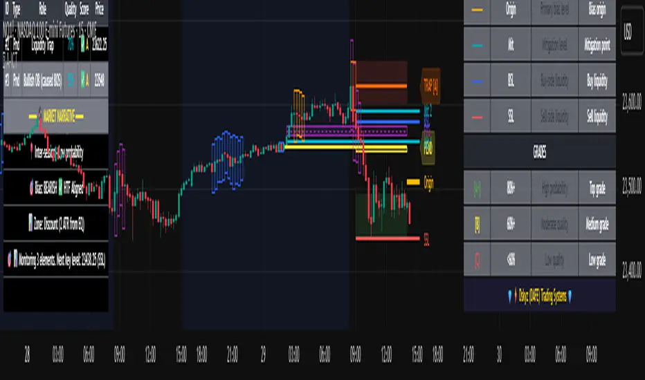
📊 THE INTELLIGENCE DASHBOARDS: YOUR COMMAND CENTER
The dashboards synthesize all the complex analysis into a simple, actionable intelligence briefing.
Main Dashboard (Bottom Right)
ICT Metrics & Breakdown: This is your statistical overview. Total Elements shows how much structure the script is tracking. High Quality instantly tells you if there are any A/B grade setups nearby. Unmitigated vs. Mitigated shows the balance of fresh opportunities versus resolved price action. The breakdown by Order Blocks, Trap Zones, etc., gives you a quick read on the market's recent character.
Structure & Market Context: This is your core bias. Order Flow tells you the current script-determined trend. Last BOS shows you the most recent structural event. CHoCH Active is a critical warning. HTF Bias shows if you are aligned with the higher timeframe—the checkmark (✓) for alignment is one of the most important confluence factors.
Smart Money Flow: A volume-based sentiment gauge. Net Flow shows the raw buying vs. selling pressure, while the Bias provides an interpretation (e.g., "STRONG BULLISH FLOW").
Key Guide (Large Dashboard only): A built-in legend so you never have to guess. It defines every pattern, structure type, and special level visually.
📖 Narrative Dashboard (Bottom Left)
This is the "story" of the market, updated in real-time. It's designed to build your trading thesis.
Recent Elements Table: A live list of the most recent, high-quality setups. It displays the Type , its Narrative Role (e.g., "Bullish OB caused BOS"), its raw Quality percentage, and its final Trade Score grade. This is your at-a-glance opportunity scanner.
Market Narrative Section: This is the soul of A-ICT. It combines all data points into a human-readable story:
📍 Current Phase: Tells you if you are in a high-volatility Killzone or a consolidation phase like the Asian Range.
🎯 Bias & Alignment: Your primary direction, with a clear indicator of HTF alignment or conflict.
🔗 Events: A causal sequence of recent events, like "💧 Sell-side liquidity swept →
📊 Bullish BOS → 🎯 Active Order Block".
🎯 Next Expectation: The script's logical conclusion. It provides a specific, forward-looking hypothesis, such as "📉 Pullback expected to bullish OB at 1.2345 before continuation up."
🎨 READING THE BATTLEFIELD: A VISUAL INTERPRETATION GUIDE
Every color and line is a piece of information. Learn to read them together to see the full picture.
The Core Zones (Boxes):
Blue Box (Order Block): Highest probability zone for trend continuation. Look for entries here.
Orange Box (Trap Zone): A manipulation footprint. Expect a potential reversal after price interacts with this zone.
Green Box (Reversal/S&R): A standard pivot area. A good reference point but requires more confluence.
Purple Box (FVG): A market imbalance. Acts as a magnet for price. An FVG inside an Order Block is an A+ confluence.
The Structural Lines:
Green/Red Line (eBOS): Confirms the trend direction. A break above the green line is bullish; a break below the red line is bearish.
Thick Orange Line (CHoCH): WARNING. The previous trend is now in question. The market character has changed.
Blue/Red Lines (BSL/SSL): Liquidity targets. Expect price to gravitate towards these lines. A dotted line with a checkmark (✓) means the liquidity has been "swept" or "purged."
How to Synthesize: The magic is in the confluence. A perfect setup might look like this: Price sweeps below a red SSL line , enters a green Discount Zone during the NY Killzone , and forms a blue Order Block which then causes a green eBOS . This sequence, visible at a glance, is the story of a high-probability long setup.
🔧 THE ARCHITECT'S VISION: THE DEVELOPMENT JOURNEY
A-ICT was forged from the frustration of using lagging indicators in a market that is forward-looking. Traditional tools are reactive; they tell you what happened. The vision for A-ICT was to create a proactive engine that could anticipate institutional behavior by understanding their objectives: liquidity and efficiency. The development process was centered on creating a "lifecycle" for price patterns—the idea that a zone's true meaning is only revealed by its consequence. This led to the post-breakout classification system and the narrative-building engine. It's designed not just to show you patterns, but to tell you their story.
⚠️ RISK DISCLAIMER & BEST PRACTICES
Advanced ICT Theory (A-ICT) is a professional-grade analytical tool and does not provide financial advice or direct buy/sell signals. Its analysis is based on historical price action and probabilities. All forms of trading involve substantial risk. Past performance is not indicative of future results. Always use this tool as part of a comprehensive trading plan that includes your own analysis and a robust risk management strategy. Do not trade based on this indicator alone.
観の目つよく、見の目よわく
"Kan no me tsuyoku, ken no me yowaku"
— Miyamoto Musashi, The Book of Five Rings
English: "Perceive that which cannot be seen with the eye."
— Dskyz, Trade with insight. Trade with anticipation.
스크립트에서 "order"에 대해 찾기
MA Crossover Strategy with TP/SL (5 EMA Filter)How the Strategy Works on a 5-Minute Chart:
Data Input (5-Minute Candles):
Every single data point (candle) on your chart will represent 5 minutes of price action (Open, High, Low, Close for that 5-minute period).
All calculations (MAs, EMA, signals) will be based on these 5-minute price data points.
Moving Average Calculations:
Fast MA (10-period SMA): This will be the Simple Moving Average of the closing prices of the last 10 five-minute candles. It reacts relatively quickly to recent price changes.
Slow MA (30-period SMA): This will be the Simple Moving Average of the closing prices of the last 30 five-minute candles. It represents a slightly longer-term trend compared to the Fast MA.
5 EMA (5-period EMA): This is the Exponential Moving Average of the closing prices of the last 5 five-minute candles. Being an EMA, it gives more weight to the most recent 5-minute prices, making it very responsive to immediate price action.
Signal Generation (Entry Conditions):
Long Entry Signal:
The 10-period SMA crosses above the 30-period SMA (indicating a potential bullish shift in the short-to-medium term trend).
AND the current 5-minute candle's closing price is above the 5-period EMA (confirming that the immediate price momentum is also bullish and supporting the crossover).
If both conditions are met at the close of a 5-minute candle, a "Buy" signal is generated.
Short Entry Signal:
The 10-period SMA crosses below the 30-period SMA (indicating a potential bearish shift).
AND the current 5-minute candle's closing price is below the 5-period EMA (confirming immediate bearish momentum).
If both conditions are met at the close of a 5-minute candle, a "Sell" signal is generated.
Trade Execution:
When a signal is triggered, the strategy enters a trade (long or short) at the closing price of that 5-minute candle.
Immediately upon entry, it places two contingent orders:
Take Profit (Target): Set at 2% (by default) away from your entry price. For a long trade, it's 2% above; for a short trade, 2% below.
Stop Loss: Set at 1% (by default) away from your entry price. For a long trade, it's 1% below; for a short trade, 1% above.
The trade will remain open until either the Take Profit or Stop Loss price is hit by subsequent 5-minute candles.
Implications for Trading on a 5-Minute Chart:
Increased Trade Frequency: You will likely see many more signals and trades compared to higher timeframes (like 1-hour or daily charts). This means more potential opportunities but also more transaction costs (commissions, slippage).
Sensitivity to Noise: Lower timeframes are more prone to "market noise" – small, random price fluctuations that don't indicate a true trend. While the 5 EMA filter helps, some false signals might still occur.
Faster Price Action: Price movements can be very rapid on a 5-minute chart. Your take profit or stop loss levels might be hit very quickly, sometimes within the same or next few candles.
Parameter Optimization is Crucial: The default MA lengths (10, 30) and EMA (5) might not be optimal for every asset or market condition on a 5-minute chart. You'll need to backtest extensively and potentially adjust these lengths, as well as the targetPerc and stopPerc, to find what works best for the specific instrument you're trading.
Risk Management: The fixed percentage stop loss is vital on a 5-minute chart due to its volatility. Without it, a few unfavorable moves could lead to significant losses.

System 0530 - Stoch RSI Strategy with ATR filterStrategy Description: System 0530 - Multi-Timeframe Stochastic RSI with ATR Filter
Overview:
This strategy, "System 0530," is designed to identify trading opportunities by leveraging the Stochastic RSI indicator across two different timeframes: a shorter timeframe for initial signal triggers (assumed to be the chart's current timeframe, e.g., 5-minute) and a longer timeframe (15-minute) for signal confirmation. It incorporates an ATR (Average True Range) filter to help ensure trades are taken during periods of adequate market volatility and includes a cooldown mechanism to prevent rapid, successive signals in the same direction. Trade exits are primarily handled by reversing signals.
How It Works:
1. Signal Initiation (e.g., 5-Minute Timeframe):
Long Signal Wait: A potential long entry is considered when the 5-minute Stochastic RSI %K line crosses above its %D line, AND the %K value at the time of the cross is at or below a user-defined oversold level (default: 30).
Short Signal Wait: A potential short entry is considered when the 5-minute Stochastic RSI %K line crosses below its %D line, AND the %K value at the time of the cross is at or above a user-defined overbought level (default: 70). When these conditions are met, the strategy enters a "waiting state" for confirmation from the 15-minute timeframe.
2. Signal Confirmation (15-Minute Timeframe):
Once in a waiting state, the strategy looks for confirmation on the 15-minute Stochastic RSI within a user-defined number of 5-minute bars (wait_window_5min_bars, default: 5 bars).
Long Confirmation:
The 15-minute Stochastic RSI %K must be greater than or equal to its %D line.
The 15-minute Stochastic RSI %K value must be below a user-defined threshold (stoch_15min_long_entry_level, default: 40).
Short Confirmation:
The 15-minute Stochastic RSI %K must be less than or equal to its %D line.
The 15-minute Stochastic RSI %K value must be above a user-defined threshold (stoch_15min_short_entry_level, default: 60).
3. Filters:
ATR Volatility Filter: If enabled, trades are only confirmed if the current ATR value (converted to ticks) is above a user-defined minimum threshold (min_atr_value_ticks). This helps to avoid taking signals during periods of very low market volatility. If the ATR condition is not met, the strategy continues to wait for the condition to be met within the confirmation window, provided other conditions still hold.
Signal Cooldown Filter: If enabled, after a signal is generated, the strategy will wait for a minimum number of bars (min_bars_between_signals) before allowing another signal in the same direction. This aims to reduce overtrading.
4. Entry and Exit Logic:
Entry: A strategy.entry() order is placed when all trigger, confirmation, and filter conditions are met.
Exit: This strategy primarily uses reversing signals for exits. For example, if a long position is open, a confirmed short signal will close the long position and open a new short position. There are no explicit take profit or stop loss orders programmed into this version of the script.
Key User-Adjustable Parameters:
Stochastic RSI Parameters: RSI Length, Stochastic RSI Length, %K Smoothing, %D Smoothing.
Signal Trigger & Confirmation:
5-minute %K trigger levels for long and short.
15-minute %K confirmation thresholds for long and short.
Wait window (in 5-minute bars) for 15-minute confirmation.
Filters:
Enable/disable and configure the Signal Cooldown filter (minimum bars between signals).
Enable/disable and configure the ATR Volatility filter (ATR period, minimum ATR value in ticks).
Strategy Parameters:
Leverage Multiplier (Note: This primarily affects theoretical position sizing for backtesting calculations in TradingView and does not simulate actual leveraged trading risks).
Recommendations for Users:
Thorough Backtesting: Test this strategy extensively on historical data for the instruments and timeframes you intend to trade.
Parameter Optimization: Experiment with different parameter settings to find what works best for your trading style and chosen markets. The default values are starting points and may not be optimal for all conditions.
Understand the Logic: Ensure you understand how each component (Stochastic RSI on different timeframes, ATR filter, cooldown) interacts to generate signals.
Risk Management: Since this version does not include explicit stop-loss orders, ensure you have a clear risk management plan in place if trading this strategy live. You might consider manually adding stop-loss orders through your broker or using TradingView's separate strategy order settings for stop-loss if applicable.
Disclaimer:
This strategy description is for informational purposes only and does not constitute financial advice. Past performance is not indicative of future results. Trading involves significant risk of loss. Always do your own research and understand the risks before trading.

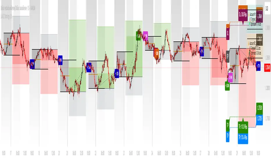
LANZ Strategy 3.0 [Backtest]🔷 LANZ Strategy 3.0 — Asian Range Fibonacci Scalping Strategy
LANZ Strategy 3.0 is a precision-engineered backtesting tool tailored for intraday traders who rely on the Asian session range to determine directional bias. This strategy implements dynamic Fibonacci projections and strict time-window validation to simulate a clean and disciplined trading environment.
🧠 Core Components:
Asian Range Bias Definition: Direction is established between 01:15–02:15 a.m. NY time based on the candle’s close in relation to the midpoint of the Asian session range (18:00–01:15 NY).
Limit Order Execution: Only one trade is placed daily, using a limit order at the Asian range high (for sells) or low (for buys), between 01:15–08:00 a.m. NY.
Fibonacci-Based TP/SL:
Original Mode: TP = 2.25x range, SL = 0.75x range.
Optimized Mode: TP = 1.95x range, SL = 0.65x range.
No Trade After 08:00 NY: If the limit order is not executed before 08:00 a.m. NY, it is canceled.
Fallback Logic at 02:15 NY: If the market direction misaligns with the setup at 02:15 a.m., the system re-evaluates and can re-issue the order.
End-of-Day Closure: All positions are closed at 15:45 NY if still open.
📊 Backtest-Ready Design:
Entries and exits are executed using strategy.entry() and strategy.exit() functions.
Position size is fixed via capital risk allocation ($100 per trade by default).
Only one position can be active at a time, ensuring controlled risk.
📝 Notes:
This strategy is ideal for assets sensitive to the Asian/London session overlap, such as Forex pairs and indices.
Easily switch between Fibonacci versions using a single dropdown input.
Fully deterministic: all entries are based on pre-defined conditions and time constraints.
👤 Credits:
Strategy developed by rau_u_lanz using Pine Script v6. Built for traders who favor clean sessions, directional clarity, and consistent execution using time-based logic and Fibonacci projections.

REVELATIONS (VoVix - PoC) REVELATIONS (VoVix - POC): True Regime Detection Before the Move
Let’s not sugarcoat it: Most strategies on TradingView are recycled—RSI, MACD, OBV, CCI, Stochastics. They all lag. No matter how many overlays you stack, every one of these “standard” indicators fires after the move is underway. The retail crowd almost always gets in late. That’s never been enough for my team, for DAFE, or for anyone who’s traded enough to know the real edge vanishes by the time the masses react.
How is this different?
REVELATIONS (VoVix - POC) was engineered from raw principle, structured to detect pre-move regime change—before standard technicals even light up. We built, tested, and refined VoVix to answer one hard question:
What if you could see the spike before the trend?
Here’s what sets this system apart, line-by-line:
o True volatility-of-volatility mathematics: It’s not just "ATR of ATR" or noise smoothing. VoVix uses normalized, multi-timeframe v-vol spikes, instantly detecting orderbook stress and "outlier" market events—before the chart shows them as trends.
o Purist regime clustering: Every trade is enabled only during coordinated, multi-filter regime stress. No more signals in meaningless chop.
o Nonlinear entry logic: No trade is ever sent just for a “good enough” condition. Every entry fires only if every requirement is aligned—local extremes, super-spike threshold, regime index, higher timeframe, all must trigger in sync.
o Adaptive position size: Your contracts scale up with event strength. Tiny size during nominal moves, max leverage during true regime breaks—never guesswork, never static exposure.
o All exits governed by regime decay logic: Trades are closed not just on price targets but at the precise moment the market regime exhausts—the hardest part of systemic trading, now solved.
How this destroys the lag:
Standard indicators (RSI, MACD, OBV, CCI, and even most “momentum” overlays) simply tell you what already happened. VoVix triggers as price structure transitions—anyone running these generic scripts will trade behind the move while VoVix gets in as stress emerges. Real alpha comes from anticipation, not confirmation.
The visuals only show what matters:
Top right, you get a live, live quant dashboard—regime index, current position size, real-time performance (Sharpe, Sortino, win rate, and wins). Bottom right: a VoVix "engine bar" that adapts live with regime stress. Everything you see is a direct function of logic driving this edge—no cosmetics, no fake momentum.
Inputs/Signals—explained carefully for clarity:
o ATR Fast Length & ATR Slow Length:
These are the heart of VoVix’s regime sensing. Fast ATR reacts to sharp volatility; Slow ATR is stability baseline. Lower Fast = reacts to every twitch; higher Slow = requires more persistent, “real” regime shifts.
Tip: If you want more signals or faster markets, lower ATR Fast. To eliminate noise, raise ATR Slow.
o ATR StdDev Window: Smoothing for volatility-of-volatility normalization. Lower = more jumpy, higher = only the cleanest spikes trigger.
Tip: Shorten for “jumpy” assets, raise for indices/futures.
o Base Spike Threshold: Think of this as your “minimum event strength.” If the current move isn’t volatile enough (normalized), no signal.
Tip: Higher = only biggest moves matter. Lower for more signals but more potential noise.
o Super Spike Multiplier: The “are you sure?” test—entry only when the current spike is this multiple above local average.
Tip: Raise for ultra-selective/swing-trading; lower for more active style.
Regime & MultiTF:
o Regime Window (Bars):
How many bars to scan for regime cluster “events.” Short for turbo markets, long for big swings/trends only.
o Regime Event Count: Only trade when this many spikes occur within the Regime Window—filters for real stress, not isolated ticks.
Tip: Raise to only ever trade during true breakouts/crashes.
o Local Window for Extremes:
How many bars to check that a spike is a local max.
Tip: Raise to demand only true, “clearest” local regime events; lower for early triggers.
o HTF Confirm:
Higher timeframe regime confirmation (like 45m on an intraday chart). Ensures any event you act on is visible in the broader context.
Tip: Use higher timeframes for only major moves; lower for scalping or fast regimes.
Adaptive Sizing:
o Max Contracts (Adaptive): The largest size your system will ever scale to, even on extreme event.
Tip: Lower for small accounts/conservative risk; raise on big accounts or when you're willing to go big only on outlier events.
o Min Contracts (Adaptive): The “toe-in-the-water.” Smallest possible trade.
Tip: Set as low as your broker/exchange allows for safety, or higher if you want to always have meaningful skin in the game.
Trade Management:
o Stop %: Tightness of your stop-loss relative to entry. Lower for tighter/safer, higher for more breathing room at cost of greater drawdown.
o Take Profit %: How much you'll hold out for on a win. Lower = more scalps. Higher = only run with the best.
o Decay Exit Sensitivity Buffer: Regime index must dip this far below the trading threshold before you exit for “regime decay.”
Tip: 0 = exit as soon as stress fails, higher = exits only on stronger confirmation regime is over.
o Bars Decay Must Persist to Exit: How long must decay be present before system closes—set higher to avoid quick fades and whipsaws.
Backtest Settings
Initial capital: $10,000
Commission: Conservative, realistic roundtrip cost:
15–20 per contract (including slippage per side) I set this to $25
Slippage: 3 ticks per trade
Symbol: CME_MINI:NQ1!
Timeframe: 1 min (but works on all timeframes)
Order size: Adaptive, 1–3 contracts
No pyramiding, no hidden DCA
Why these settings?
These settings are intentionally strict and realistic, reflecting the true costs and risks of live trading. The 10,000 account size is accessible for most retail traders. 25/contract including 3 ticks of slippage are on the high side for NQ, ensuring the strategy is not curve-fit to perfect fills. If it works here, it will work in real conditions.
Tip: Set to 1 for instant regime exit; raise for extra confirmation (less whipsaw risk, exits held longer).
________________________________________
Bottom line: Tune the sensitivity, selectivity, and risk of REVELATIONS by these inputs. Raise thresholds and windows for only the best, most powerful signals (institutional style); lower for activity (scalpers, fast cryptos, signals in constant motion). Sizing is always adaptive—never static or martingale. Exits are always based on both price and regime health. Every input is there for your control, not to sell “complexity.” Use with discipline, and make it your own.
This strategy is not just a technical achievement: It’s a statement about trading smarter, not just more.
* I went back through the code to make sure no the strategy would not suffer from repainting, forward looking, or any frowned upon loopholes.
Disclaimer:
Trading is risky and carries the risk of substantial loss. Do not use funds you aren’t prepared to lose. This is for research and informational purposes only, not financial advice. Backtest, paper trade, and know your risk before going live. Past performance is not a guarantee of future results.
Expect more: We’ll keep pushing the standard, keep evolving the bar until “quant” actually means something in the public code space.
Use with clarity, use with discipline, and always trade your edge.
— Dskyz , for DAFE Trading Systems

15-Min Opening Range Breakout STEP-BY-STEP RULES
1. Define the Opening Range (OR)
Mark the high and low of the first 15-minute candle of the session.
This creates your Opening Range.
Example: London session opens at 08:00 GMT. Use the 08:00–08:15 candle.
2. Set Entry Triggers
Buy Breakout: Place a Buy Stop order 1 pip above the Opening Range high.
Sell Breakout: Place a Sell Stop order 1 pip below the Opening Range low.
⚠️ Only one side should be triggered. Cancel the opposite order once one is active.
3. Set Stop Loss (SL)
For Buy trades:
SL = Opening Range Low - 2 pips
For Sell trades:
SL = Opening Range High + 2 pips
This ensures you give the price enough space, while keeping risk controlled.
4. Set Take Profit (TP)
Use either of these two approaches:
✅ Fixed Risk-Reward (Preferred)
Target 1: TP = 2R (i.e., 2 × SL distance)
Target 2 (optional): Leave runner for 3R or trail stop behind minor S/R
✅ Fixed Pip Target (alternative)
TP = +50 pips
SL = -20 pips
Matches your preferred risk model of 20 SL / 50 TP
5. Trade Management
If no breakout occurs within 1 hour, cancel the pending orders. No trade that day.
If trade triggers but fails to move, consider time-based exit after 2 hours.
Optional: Move SL to breakeven once price moves 1R in your favor.

LANZ Strategy 3.0🔷 LANZ Strategy 3.0 — Asian Range Fibonacci Strategy with Execution Window Logic
LANZ Strategy 3.0 is a rule-based trading system that utilizes the Asian session range to project Fibonacci levels and manage entries during a defined execution window. Designed for Forex and index traders, this strategy focuses on structured price behavior around key levels before the New York session.
🧠 Core Components:
Asian Session Range Mapping: Automatically detects the high, low, and midpoint during the Asian session.
Fibonacci Level Projection: Projects configurable Fibonacci retracement and extension levels based on the Asian range.
Execution Window Logic: Uses the 01:15 NY candle as a reference to validate potential reversals or continuation setups.
Conditional Entry System: Includes logic for limit order entries (buy or sell) at specific Fib levels, with reversal logic if price breaks structure before execution.
Risk Management: Entry orders are paired with dynamic SL and TP based on Fibonacci-based distances, maintaining a risk-reward ratio consistent with intraday strategies.
📊 Visual Features:
Asian session high/low/mid lines.
Fibonacci levels: Original (based on raw range) and Optimized (user-adjustable).
Session background coloring for Asia, Execution Window, and NY session.
Labels and lines for entry, SL, and TP targets.
Dynamic deletion of untriggered orders after execution window expires.
⚙️ How It Works:
The script calculates the Asian session range.
Projects Fibonacci levels from the range.
Waits for the 01:15 NY candle to close to validate a signal.
If valid, a limit entry order (BUY or SELL) is plotted at the selected level.
If price structure changes (e.g., breaks the high/low), reversal logic may activate.
If no trade is triggered, orders are cleared before the NY session.
🔔 Alerts:
Alerts trigger when a valid setup appears after 01:15 NY candle.
Optional alerts for order activation, SL/TP hit, or trade cancellation.
📝 Notes:
Intended for semi-automated or discretionary trading.
Best used on highly liquid markets like Forex majors or indices.
Script parameters include session times, Fib ratios, SL/TP settings, and reversal logic toggle.
Credits:
Developed by LANZ, this script merges traditional session-based analysis with Fibonacci tools and structured execution timing, offering a unique framework for morning volatility plays.
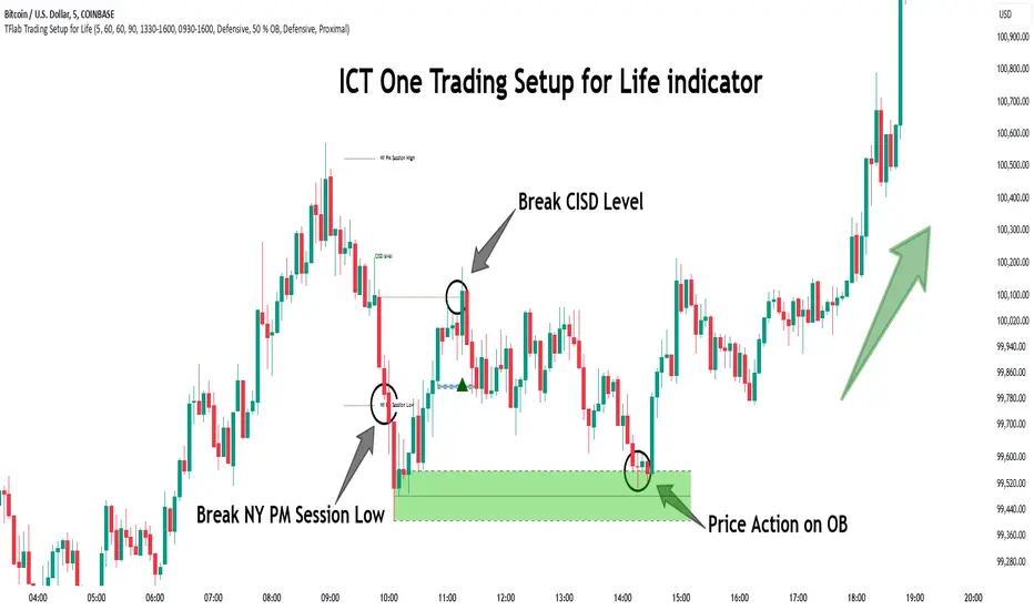
One Trading Setup for Life ICT [TradingFinder] Sweep Session FVG🔵 Introduction
ICT One Trading Setup for Life is a trading strategy based on liquidity and market structure shifts, utilizing the PM Session Sweep to determine price direction. In this strategy, the market first forms a price range during the PM Session (from 13:30 to 16:00 EST), which includes the highest high (PM Session High) and lowest low (PM Session Low).
In the next session, the price first touches one of these levels to trigger a Liquidity Hunt before confirming its trend by breaking the Change in State of Delivery (CISD) Level. After this confirmation, the price retraces toward a Fair Value Gap (FVG) or Order Block (OB), which serve as the best entry points in alignment with liquidity.
In financial markets, liquidity is the primary driver of price movement, and major market participants such as institutional investors and banks are constantly seeking liquidity at key levels. This process, known as Liquidity Hunt or Liquidity Sweep, occurs when the price reaches an area with a high concentration of orders, absorbs liquidity, and then reverses direction.
In this setup, the PM Session range acts as a trading framework, where its highs and lows function as key liquidity zones that influence the next session’s price movement. After the New York market opens at 9:30 EST, the price initially breaks one of these levels to capture liquidity.
However, for a trend shift to be confirmed, the CISD Level must be broken.
Once the CISD Level is breached, the price retraces toward an FVG or OB, which serve as optimal trade entry points.
Bullish Setup :
Bearish Setup :
🔵 How to Use
In this strategy, the PM Session range is first identified, which includes the highest high (PM Session High) and lowest low (PM Session Low) between 13:30 and 16:00 EST. In the following session, the price touches one of these levels for a Liquidity Hunt, followed by a break of the Change in State of Delivery (CISD) Level. The price then retraces toward a Fair Value Gap (FVG) or Order Block (OB), creating a trading opportunity.
This process can occur in two scenarios : bearish and bullish setups.
🟣 Bullish Setup
In a bullish scenario, the PM Session High and PM Session Low are identified. In the following session, the price first breaks the PM Session Low, absorbing liquidity. This process results in a Fake Breakout to the downside, misleading retail traders into taking short positions.
After the Liquidity Hunt, the CISD Level is broken, confirming a trend reversal. The price then retraces toward an FVG or OB, offering an optimal long entry opportunity.
The initial take-profit target is the PM Session High, but if higher timeframe liquidity levels exist, extended targets can be set.
The stop-loss should be placed below the Fake Breakout low or the first candle of the FVG.
🟣 Bearish Setup
In a bearish scenario, the market first defines its PM Session High and PM Session Low. In the next session, the price initially breaks the PM Session High, triggering a Liquidity Hunt. This movement often causes a Fake Breakout, misleading retail traders into taking incorrect positions.
After absorbing liquidity, the CISD Level breaks, indicating a shift in market structure. The price then retraces toward an FVG or OB, offering the best short entry opportunity.
The initial take-profit target is the PM Session Low, but if additional liquidity exists on higher timeframes, lower targets can be considered.
The stop-loss should be placed above the Fake Breakout high or the first candle of the FVG.
🔵 Setting
CISD Bar Back Check : The Bar Back Check option enables traders to specify the number of past candles checked for identifying the CISD Level, enhancing CISD Level accuracy on the chart.
Order Block Validity : The number of candles that determine the validity of an Order Block.
FVG Validity : The duration for which a Fair Value Gap remains valid.
CISD Level Validity : The duration for which a CISD Level remains valid after being broken.
New York PM Session : Defines the PM Session range from 13:30 to 16:00 EST.
New York AM Session : Defines the AM Session range from 9:30 to 16:00 EST.
Refine Order Block : Enables finer adjustments to Order Block levels for more accurate price responses.
Mitigation Level OB : Allows users to set specific reaction points within an Order Block, including: Proximal: Closest level to the current price. 50% OB: Midpoint of the Order Block. Distal: Farthest level from the current price.
FVG Filter : The Judas Swing indicator includes a filter for Fair Value Gap (FVG), allowing different filtering based on FVG width: FVG Filter Type: Can be set to "Very Aggressive," "Aggressive," "Defensive," or "Very Defensive." Higher defensiveness narrows the FVG width, focusing on narrower gaps.
Mitigation Level FVG : Like the Order Block, you can set price reaction levels for FVG with options such as Proximal, 50% OB, and Distal.
Demand Order Block : Enables or disables bullish Order Block.
Supply Order Block : Enables or disables bearish Order Blocks.
Demand FVG : Enables or disables bullish FVG.
Supply FVG : Enables or disables bearish FVGs.
Show All CISD : Enables or disables the display of all CISD Levels.
Show High CISD : Enables or disables high CISD levels.
Show Low CISD : Enables or disables low CISD levels.
🔵 Conclusion
The ICT One Trading Setup for Life is a liquidity-based strategy that leverages market structure shifts and precise entry points to identify high-probability trade opportunities. By focusing on PM Session High and PM Session Low, this setup first captures liquidity at these levels and then confirms trend shifts with a break of the Change in State of Delivery (CISD) Level.
Entering a trade after a retracement to an FVG or OB allows traders to position themselves at optimal liquidity levels, ensuring high reward-to-risk trades. When used in conjunction with higher timeframe bias, order flow, and liquidity analysis, this strategy can become one of the most effective trading methods within the ICT Concept framework.
Successful execution of this setup requires risk management, patience, and a deep understanding of liquidity dynamics. Traders can enhance their confidence in this strategy by conducting extensive backtesting and analyzing past market data to optimize their approach for different assets.
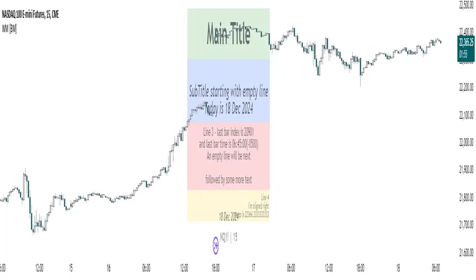
Watermark with dynamic variables [BM]█ OVERVIEW
This indicator allows users to add highly customizable watermark messages to their charts. Perfect for branding, annotation, or displaying dynamic chart information, this script offers advanced customization options including dynamic variables, text formatting, and flexible positioning.
█ CONCEPTS
Watermarks are overlay messages on charts. This script introduces placeholders — special keywords wrapped in % signs — that dynamically replace themselves with chart-related data. These watermarks can enhance charts with context, timestamps, or branding.
█ FEATURES
Dynamic Variables : Replace placeholders with real-time data such as bar index, timestamps, and more.
Advanced Customization : Modify text size, color, background, and alignment.
Multiple Messages : Add up to four independent messages per group, with two groups supported (A and B).
Positioning Options : Place watermarks anywhere on the chart using predefined locations.
Timezone Support : Display timestamps in a preferred timezone with customizable formats.
█ INPUTS
The script offers comprehensive input options for customization. Each Watermark (A and B) contains identical inputs for configuration.
Watermark settings are divided into two levels:
Watermark-Level Settings
These settings apply to the entire watermark group (A/B):
Show Watermark: Toggle the visibility of the watermark group on the chart.
Position: Choose where the watermark group is displayed on the chart.
Reverse Line Order: Enable to reverse the order of the lines displayed in Watermark A.
Message-Level Settings
Each watermark contains up to four configurable messages. These messages can be independently customized with the following options:
Message Content: Enter the custom text to be displayed. You can include placeholders for dynamic data.
Text Size: Select from predefined sizes (Tiny, Small, Normal, Large, Huge) or specify a custom size.
Text Alignment and Colors:
- Adjust the alignment of the text (Left, Center, Right).
- Set text and background colors for better visibility.
Format Time: Enable time formatting for this watermark message and configure the format and timezone. The settings for each message include message content, text size, alignment, and more. Please refer to Formatting dates and times for more details on valid formatting tokens.
█ PLACEHOLDERS
Placeholders are special keywords surrounded by % signs, which the script dynamically replaces with specific chart-related data. These placeholders allow users to insert dynamic content, such as bar information or timestamps, into watermark messages.
Below is the complete list of currently available placeholders:
bar_index , barstate.isconfirmed , barstate.isfirst , barstate.ishistory , barstate.islast , barstate.islastconfirmedhistory , barstate.isnew , barstate.isrealtime , chart.is_heikinashi , chart.is_kagi , chart.is_linebreak , chart.is_pnf , chart.is_range , chart.is_renko , chart.is_standard , chart.left_visible_bar_time , chart.right_visible_bar_time , close , dayofmonth , dayofweek , dividends.future_amount , dividends.future_ex_date , dividends.future_pay_date , earnings.future_eps , earnings.future_period_end_time , earnings.future_revenue , earnings.future_time , high , hl2 , hlc3 , hlcc4 , hour , last_bar_index , last_bar_time , low , minute , month , ohlc4 , open , second , session.isfirstbar , session.isfirstbar_regular , session.islastbar , session.islastbar_regular , session.ismarket , session.ispostmarket , session.ispremarket , syminfo.basecurrency , syminfo.country , syminfo.currency , syminfo.description , syminfo.employees , syminfo.expiration_date , syminfo.industry , syminfo.main_tickerid , syminfo.mincontract , syminfo.minmove , syminfo.mintick , syminfo.pointvalue , syminfo.prefix , syminfo.pricescale , syminfo.recommendations_buy , syminfo.recommendations_buy_strong , syminfo.recommendations_date , syminfo.recommendations_hold , syminfo.recommendations_sell , syminfo.recommendations_sell_strong , syminfo.recommendations_total , syminfo.root , syminfo.sector , syminfo.session , syminfo.shareholders , syminfo.shares_outstanding_float , syminfo.shares_outstanding_total , syminfo.target_price_average , syminfo.target_price_date , syminfo.target_price_estimates , syminfo.target_price_high , syminfo.target_price_low , syminfo.target_price_median , syminfo.ticker , syminfo.tickerid , syminfo.timezone , syminfo.type , syminfo.volumetype , ta.accdist , ta.iii , ta.nvi , ta.obv , ta.pvi , ta.pvt , ta.tr , ta.vwap , ta.wad , ta.wvad , time , time_close , time_tradingday , timeframe.isdaily , timeframe.isdwm , timeframe.isintraday , timeframe.isminutes , timeframe.ismonthly , timeframe.isseconds , timeframe.isticks , timeframe.isweekly , timeframe.main_period , timeframe.multiplier , timeframe.period , timenow , volume , weekofyear , year
█ HOW TO USE
1 — Add the Script:
Apply "Watermark with dynamic variables " to your chart from the TradingView platform.
2 — Configure Inputs:
Open the script settings by clicking the gear icon next to the script's name.
Customize visibility, message content, and appearance for Watermark A and Watermark B.
3 — Utilize Placeholders:
Add placeholders like %bar_index% or %timenow% in the "Watermark - Message" fields to display dynamic data.
Empty lines in the message box are reflected on the chart, allowing you to shift text up or down.
Using \n in the message box translates to a new line on the chart.
4 — Preview Changes:
Adjust settings and view updates in real-time on your chart.
█ EXAMPLES
Branding
DodgyDD's charts
Debugging
█ LIMITATIONS
Only supports variables defined within the script.
Limited to four messages per watermark.
Visual alignment may vary across different chart resolutions or zoom levels.
Placeholder parsing relies on correct input formatting.
█ NOTES
This script is designed for users seeking enhanced chart annotation capabilities. It provides tools for dynamic, customizable watermarks but is not a replacement for chart objects like text labels or drawings. Please ensure placeholders are properly formatted for correct parsing.
Additionally, this script can be a valuable tool for Pine Script developers during debugging . By utilizing dynamic placeholders, developers can display real-time values of variables and chart data directly on their charts, enabling easier troubleshooting and code validation.
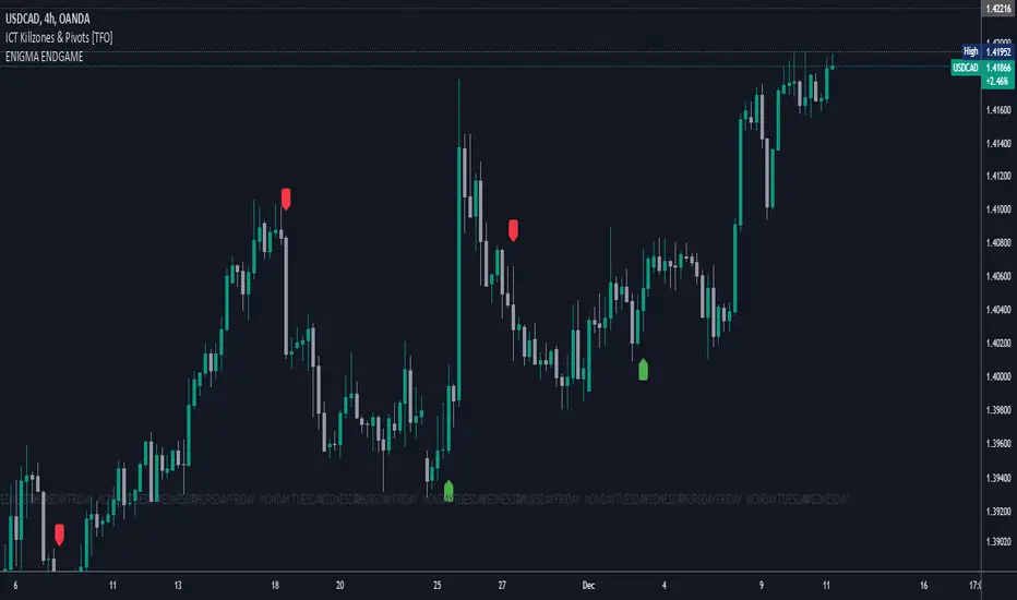
Enigma End Game Indicator
Enigma End Game Indicator Description
The Enigma End Game indicator is a powerful tool designed to enhance the way traders approach support and resistance, combining mainstream technical analysis with a unique, dynamic perspective. At its core, this indicator enables traders to adapt to market conditions in real time by applying a blend of classic and modern interpretations of support and resistance levels.
In traditional support and resistance analysis, we recognize the significant price points where the market has historically reversed or consolidated. However, the *Enigma End Game* indicator takes this one step further by analyzing each individual candle's high as a potential resistance level and each low as support. This allows the trader to stay more agile, as the market constantly updates and evolves. The dynamic nature of this method acknowledges that price movements are fractal in nature, meaning that these levels are not static but adjust in response to price action on multiple timeframes.
### How It Works:
When using the *Enigma End Game* indicator, it doesn't simply plot buy and sell signals automatically. Instead, the indicator highlights key levels based on the interaction between price and historical price action. Here's how it operates:
1. **Buy Logic:**
The indicator identifies bullish signals based on the *Enigma* logic, but it does not trigger an immediate buy. Instead, it plots arrows above or below the candles, indicating the key price levels where price action has shifted. Traders then focus on these areas, particularly looking for buy opportunities *below* these levels during key market sessions (such as London or New York) while aligning with both mainstream support and resistance and *Enigma* levels.
2. **Sell Logic:**
Similarly, when the indicator identifies a sell signal, it plots an arrow above the candle where price action has reversed. This does not immediately suggest selling. Traders wait for a price retracement back to the previously breached low (for a sell order) or high (for a buy order), observing price action closely on lower timeframes (such as the 1-minute chart) to refine entry points. The entry is triggered when price starts to show signs of reversing at these levels, further validated by mainstream and *Enigma* support/resistance.
### Practical Example – XAU/USD (Gold):
For instance, in the settings of the *Enigma End Game* indicator, if we select the 5-minute (5MN) timeframe as the key level, the indicator will only plot the first 3 arrows following the *Enigma* logic. The arrows will appear above or below the candle that was breached, indicating a potential trend reversal. In this scenario, the first arrow marks the point where price broke a significant support or resistance level. Afterward, the trader watches for a subsequent candle to close below (in the case of a sell) the previous candle’s low, confirming a bearish bias.
Now, the trader does not rush into a sell order. Instead, they wait for the price to pull back towards the previously breached low. At this point, the trader can use a lower timeframe (like the 1-minute chart) to identify both mainstream support and resistance levels and *Enigma* levels above the main 5-minute key level. These additional levels provide a clearer understanding of where price might reverse and give the trader a stronger edge in refining their entry point.
The trader then sets a sell order *above* the price level of the previous low, but only once signs show that price is retracing and ready to fall again. The price point where this retracement occurs, confirmed by both mainstream and *Enigma* levels, becomes the entry signal for the trade.
### Summary:
The *Enigma End Game* indicator combines time-tested principles of support and resistance with a more modern, adaptive view, empowering traders to read the market with greater precision. It guides you to wait for optimal entries, based on dynamic support and resistance levels that change with each price movement. By combining signals on higher timeframes with refined entries on lower timeframes, traders gain a unique advantage in navigating both obvious and hidden levels of support and resistance, ultimately improving their ability to time trades with higher probability of success.
This indicator allows for a more calculated, strategic approach to trading—highlighting the right moments to enter the market while providing the flexibility to adjust to different market conditions.
The *ENIGMA Signals with Retests* indicator is a versatile trading tool that combines key market sessions with dynamic support and resistance levels. It uses logic to identify potential buy and sell signals based on the behavior of recent price swings (highs and lows) and offers flexibility with the number of arrows plotted per session. The user can customize settings like arrow frequency, line styles, and session times, allowing for personalized trading strategies.
The indicator detects buy and sell signals by checking if the price breaks the previous swing high (for buy signals) or swing low (for sell signals). It then stores these levels and draws horizontal lines on the chart, representing critical price levels where traders can expect potential price reactions.
A key feature of this indicator is its ability to limit the number of arrows per session, ensuring a cleaner chart and reducing signal clutter. Horizontal lines are drawn at the identified buy or sell levels, with the option to display labels like "BUY - AT OR BELOW" and "SELL - AT OR ABOVE" to further clarify entry points.
The indicator also incorporates session filtering, allowing traders to focus on specific market sessions (Asia, London, and New York) for more relevant signals, and it ensures that no more than a user-defined number of arrows are plotted within a session.
3 CANDLE SUPPLY/DEMANDExplanation of the Code:
Demand Zone Logic: The script checks if the second candle closes below the low of the first candle and the third candle closes above both the highs of the first and second candles.
Zone Plotting: Once the pattern is identified, a demand zone is plotted from the low of the first candle to the high of the third candle, using a dashed green line for clarity.
Markers: A small triangle marker is added below the bars where a demand zone is detected for easy visualization.
Efficient Logic: The script checks the conditions for demand zone formation for every three consecutive candles on the chart.
This approach should be both accurate and efficient in plotting demand zones, making it easier to spot potential support levels on the chart.

MFI Strategy with Oversold Zone Exit and AveragingThis strategy is based on the Money Flow Index (MFI) and aims to enter a long position when the MFI exits an oversold zone, with specific rules for limit orders, stop-loss, and take-profit settings. Here's a detailed breakdown:
Key Components
1. **Money Flow Index (MFI)**: The strategy uses the MFI, a volume-weighted indicator, to gauge whether the market is in an oversold condition (default threshold of MFI < 20). Once the MFI rises above the oversold threshold, it signals a potential buying opportunity.
2. **Limit Order for Long Entry**: Instead of entering immediately after the oversold condition is cleared, the strategy places a limit order at a price slightly below the current price (by a user-defined percentage). This helps achieve a better entry price.
3. **Stop-Loss and Take-Profit**:
- **Stop-Loss**: A stop-loss is set to protect against significant losses, calculated as a percentage below the entry price.
- **Take-Profit**: A take-profit target is set as a percentage above the entry price to lock in gains.
4. **Order Cancellation**: If the limit order isn’t filled within a specific number of bars (default is 5 bars), it’s automatically canceled to avoid being filled at a potentially suboptimal price as market conditions change.
Strategy Workflow
1. **Identify Oversold Zone**: The strategy checks if the MFI falls below a defined oversold level (default is 20). Once this condition is met, the flag `inOversoldZone` is set to `true`.
2. **Wait for Exit from Oversold Zone**: When the MFI rises back above the oversold level, it’s considered a signal that the market is potentially recovering, and the strategy prepares to enter a position.
3. **Place Limit Order**: Upon exiting the oversold zone, the strategy places a limit order for a long position at a price below the current price, defined by the `Long Entry Percentage` parameter.
4. **Monitor Limit Order**: A counter (`barsSinceEntryOrder`) starts counting the bars since the limit order was placed. If the order isn’t filled within the specified number of bars, it’s canceled automatically.
5. **Set Stop-Loss and Take-Profit**: Once the order is filled, a stop-loss and take-profit are set based on user-defined percentages relative to the entry price.
6. **Exit Strategy**: The trade will close automatically when either the stop-loss or take-profit level is hit.
Advantages
- **Risk Management**: With configurable stop-loss and take-profit, the strategy ensures losses are limited while capturing profits at pre-defined levels.
- **Controlled Entry**: The use of a limit order below the current price helps secure a better entry point, enhancing risk-reward.
- **Oversold Exit Trigger**: Using the exit from an oversold zone as an entry condition can help catch reversals.
Disadvantages
- **Missed Entries**: If the limit order isn’t filled due to insufficient downward movement after the oversold signal, potential opportunities may be missed.
- **Dependency on MFI Sensitivity**: As the MFI is sensitive to both price and volume, its fluctuations might not always accurately represent oversold conditions.
Overall Purpose
The strategy is suited for traders who want to capture potential reversals after oversold conditions in the market, with a focus on precise entries, risk management, and an automated exit plan.

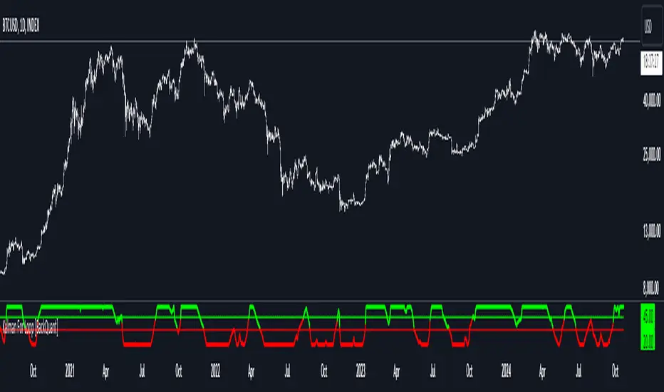
Kalman For Loop [BackQuant]Kalman For Loop
Introducing BackQuant's Kalman For Loop (Kalman FL) — a highly adaptive trading indicator that uses a Kalman filter to smooth price data and generate actionable long and short signals. This advanced indicator is designed to help traders identify trends, filter out market noise, and optimize their entry and exit points with precision. Let’s explore how this indicator works, its key features, and how it can enhance your trading strategies.
Core Concept: Kalman Filter
The Kalman Filter is a mathematical algorithm used to estimate the state of a system by filtering noisy data. It is widely used in areas such as control systems, signal processing, and time-series analysis. In the context of trading, a Kalman filter can be applied to price data to smooth out short-term fluctuations, providing a clearer view of the underlying trend.
Unlike moving averages, which use fixed weights to smooth data, the Kalman Filter adjusts its estimate dynamically based on the relationship between the process noise and the measurement noise. This makes the filter more adaptive to changing market conditions, providing more accurate trend detection without the lag associated with traditional smoothing techniques.
Please see the original Kalman Price Filter
In this script, the Kalman For Loop applies the Kalman filter to the price source (default set to the closing price) to generate a smoothed price series, which is then used to calculate signals.
Adaptive Smoothing with Process and Measurement Noise
Two key parameters govern the behavior of the Kalman filter:
Process Noise: This controls the extent to which the model allows for uncertainty in price changes. A lower process noise value will make the filter smoother but slower to react to price changes, while a higher value makes it more sensitive to recent price fluctuations.
Measurement Noise: This represents the uncertainty or "noise" in the observed price data. A higher measurement noise value gives the filter more leeway to ignore short-term fluctuations, focusing on the broader trend. Lowering the measurement noise makes the filter more responsive to minor changes in price.
These settings allow traders to fine-tune the Kalman filter’s sensitivity, adjusting it to match their preferred trading style or market conditions.
For-Loop Scoring Mechanism
The Kalman FL further enhances the effectiveness of the Kalman filter by using a for-loop scoring system. This mechanism evaluates the smoothed price over a range of periods (defined by the Calculation Start and Calculation End inputs), assigning a score based on whether the current filtered price is higher or lower than previous values.
Long Signals: A long signal is generated when the for-loop score surpasses the Long Threshold (default set at 20), indicating a strong upward trend. This helps traders identify potential buying opportunities.
Short Signals: A short signal is triggered when the score crosses below the Short Threshold (default set at -10), signaling a potential downtrend or selling opportunity.
These signals are plotted on the chart, giving traders a clear visual indication of when to enter long or short positions.
Customization and Visualization Options
The Kalman For Loop comes with a range of customization options to give traders full control over how the indicator operates and is displayed on the chart:
Kalman Price Source: Choose the price data used for the Kalman filter (default is the closing price), allowing you to apply the filter to other price points like open, high, or low.
Filter Order: Set the order of the Kalman filter (default is 5), controlling how far back the filter looks in its calculations.
Process and Measurement Noise: Fine-tune the sensitivity of the Kalman filter by adjusting these noise parameters.
Signal Line Width and Colors: Customize the appearance of the signal line and the colors used to indicate long and short conditions.
Threshold Lines: Toggle the display of the long and short threshold lines on the chart for better visual clarity.
The indicator also includes the option to color the candlesticks based on the current trend direction, allowing traders to quickly identify changes in market sentiment. In addition, a background color feature further highlights the overall trend by shading the background in green for long signals and red for short signals.
Trading Applications
The Kalman For Loop is a versatile tool that can be adapted to a variety of trading strategies and markets. Some of the primary use cases include:
Trend Following: The adaptive nature of the Kalman filter helps traders identify the start of new trends with greater precision. The for-loop scoring system quantifies the strength of the trend, making it easier to stay in trades for longer when the trend remains strong.
Mean Reversion: For traders looking to capitalize on short-term reversals, the Kalman filter's ability to smooth price data makes it easier to spot when price has deviated too far from its expected path, potentially signaling a reversal.
Noise Reduction: The Kalman filter excels at filtering out short-term price noise, allowing traders to focus on the broader market movements without being distracted by minor fluctuations.
Risk Management: By providing clear long and short signals based on filtered price data, the Kalman FL helps traders manage risk by entering positions only when the trend is well-defined, reducing the chances of false signals.
Alerts and Automation
To further assist traders, the Kalman For Loop includes built-in alert conditions that notify you when a long or short signal is generated. These alerts can be configured to trigger notifications, helping you stay on top of market movements without constantly monitoring the chart.
Final Thoughts
The Kalman For Loop is a powerful and adaptive trading indicator that combines the precision of the Kalman filter with a for-loop scoring mechanism to generate reliable long and short signals. Whether you’re a trend follower or a reversal trader, this indicator offers the flexibility and accuracy needed to navigate complex markets with confidence.
As always, it’s important to backtest the indicator and adjust the settings to fit your trading style and market conditions. No indicator is perfect, and the Kalman FL should be used alongside other tools and sound risk management practices for the best results.
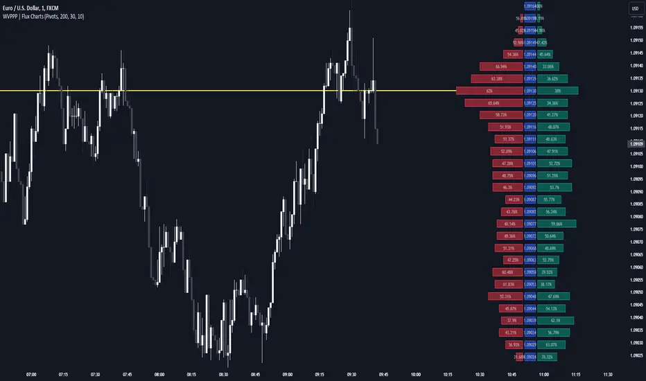
Weighted Volume Profile Pivot Points | Flux Charts💎 GENERAL OVERVIEW
Introducing our new Weighted Volume Profile Pivot Points (WVPPP) Indicator! This indicator renders a volume profile using the latest pivot points, automatically adjusting itself when new pivots occur. The pivoting mode can be switched between default pivot points and order blocks mode. It can be adjusted to give more weight to recent or past candlesticks, or can be used as a normal volume profile. For more information, please read the full write-up.
Features of the new Weighted Volume Profile Pivot Points (WVPPP) Indicator :
Renders Volume Profile Of The Range Between Latest Pivots
Two Pivoting Modes Including Order Blocks Mode
Adjustable Weighthing Towards Past or Recent
Customizable Row Count & Maximum Distance
Left or Right Alignment
More Styling Options
🚩UNIQUENESS
This indicator stands out with two key features. One is it's ability to weight volumes based on their distance to the current time. Giving weight to volumes may offer new trading opportunities to traders as they can now see the most recent Point Of Control (POC) or a more powerful but past POC based on their choice. Another key feature the indicator has is that it automatically finds latest valid pivot points, and uses that range for the volume profile. The range changes dynamically as new pivots points emerge. You can select between normal pivot points and order blocks mode. The indicator also has a variety of useful styling settings such as aligning the volume profile to the right or the left of the chart, POC Line styling and color settings for bullish & bearish volumes.
📌 HOW DOES IT WORK ?
A volume profile provides an in-depth look at trading activity over a period of time by plotting a histogram on the price axis. This indicator can also give weight to volumes based on their distance to the current time, essentially determining their importance for the profile. The range which the volume profile will cover is determined by the latest pivot points. Here is how it works step-by-step :
1. Determine how much candlesticks the volume profile will cover (Analyze Bars setting)
2. Find the latest pivot points. If the mode is set to "Pivots", the pivot points are the candlesticks which has the highest / lowest wick in X amount of bars (Swing Length setting). If the mode is set to "Order Blocks", the volume profile range is the area between the latest buyside order block and the sellside order block. Order blocks occur when there is a high amount of market orders exist on a price range. It is possible to find order blocks using specific candlestick formations on the chart. For more information about the order block detection, I suggest you checking the write-up of our "Volumized Order Blocks" script. Increasing the "Swing Length" setting is recommended when the mode is set to "Pivots", as this will help in finding stronger pivot points.
3. Make a range using the latest pivot points, then divide it into rows (Row Count setting)
4. Then for each candlestick, add it's volume to the corresponding row in the range. Note that the volume can be added into several rows if it overlaps with them all.
5. If the candlestick is a bullish candlestick, we add it's volume into the bullish volume of the row, if it's a bearish candlestick, we add it to the bearish volume of the row.
With the weighted volume mode, which is activated if "Volume Weighthing" setting is set to "Recent" or "Past", all volumes get a penalty based on their distance to the latest candletstick. For example, if the setting is set to "Recent", the latest candlestick contributes it's volume by 100% to the corresponding row, but the candlestick which is 50 candlesticks far from the current candlestick only contributes it's volume by ~17% to the row. The same applies to the "Past" setting, but in the reversed order, where past candlesticks have more priority than the current ones.
Volume contribution percent for "Recent" setting : ((100 * 0.85) / (i + 1)) + (100 * (1.0 - 0.85))
Volume contribution percent for "Past" setting : ((100 * 0.85) * ((i + 1) / N)) + (100 * (1.0 - 0.85))
Where i = candlestick index from right to left, N = total number of candlesticks analyzed by the volume profile.
The Point Of Control (POC) line is drawn from the row with the most total volume, and is generally considered as a strong level because a lot of trading volume happened on that particular row. Traders may use this line as a support & resistance level.
We believe that automatically ranging the volume profile to important pivot points will help traders see crucial volume information easier without unnecessary hassle. Traders can use this indicator to have an insight of areas which price moves quickly without much volume, or see areas that holds the price still for much longer and plan their trades accordingly.
⚙️SETTINGS
1. General Configuration
Mode -> The pivoting mode that is switchable between "Pivots" and "Order Blocks" as described in the write-up. Please read the upper section to understand how this setting works.
Analyze Bars -> Total amount of bars that will be analyzed by the indicator from right to left.
Row Count -> The amount of rows that will the vertical range between pivot points will be divided into.
Volume Weighting -> The volume weighting mode as explained in the write-up.
2. Style
Highlight Sessions -> The volume profile sessions will be highlighted with a blue tint. To prevent confusion, highlighting will not work if the alignment is set to "Right".
Align To -> The alignment of the volume profile.
Alligator + MA Trend Catcher [TradeDots]The "Alligator + MA Trend Catcher" is a trading strategy that integrates the William Alligator indicator with a Moving Average (MA) to establish robust entry and exit conditions, optimized for capturing trends.
HOW IT WORKS
This strategy combines the traditional William Alligator set up with an additional Moving Average indicator for enhanced trend confirmation, creating a user-friendly backtesting tool for traders who prefer the Alligator method.
The original Alligator strategy can frequently present fluctuations, even in well-established trends, leading to potentially premature exits. To mitigate this, we incorporate a Moving Average as a secondary confirmation measure to ensure the market trend has indeed shifted.
Here’s the operational flow for long orders:
Entry Signal: When the price rises above the Moving Average, it confirms a bullish market state. Enter if Alligator spread in an upward direction. The trade remains active even if the Alligator indicator suggests a trend reversal.
Exit Signal: The position is closed when the price falls below the Moving Average, and the Alligator spreads in the downward direction. This setup helps traders to maintain positions through the entirety of the trend for maximum gain.
APPLICATION
This strategy is tailored for assets with significant, well-defined trends, such as Bitcoin and Ethereum, which are known for their high volatility and substantial price movements.
This strategy offers a low win-rate but high reward configuration, making asset selection critical for long-term profitability. If you choose assets that lack strong price momentum, there's a high chance that this strategy may not be effective.
For traders seeking to maximize gains from large trends without exiting prematurely, this strategy provides an aggressive yet controlled approach to riding out substantial market waves.
DEFAULT SETUP
Commission: 0.01%
Initial Capital: $10,000
Equity per Trade: 80%
RISK DISCLAIMER
Trading entails substantial risk, and most day traders incur losses. All content, tools, scripts, articles, and education provided by TradeDots serve purely informational and educational purposes. Past performances are not definitive predictors of future results.

Fractional Differentiation█ Description
This Pine Script indicator implements fractional differentiation, a mathematical operation that extends the concept of differentiation to non-integer orders. Fractional differentiation is particularly significant in financial analysis, as it enables analysts to uncover underlying patterns in price series that are not evident with traditional integer-order differentiation. The motivation behind fractional differencing lies in its ability to balance the trade-off between retaining data/feature memory and ensuring stationarity.
█ Significance
Fractional differentiation offers a nuanced view of market data, allowing for the adjustment of the differentiation order to balance between signal clarity and noise reduction. This is especially useful in financial markets, where the choice of differentiation order can highlight long-term trends or short-term price movements without completely smoothing out the valuable market noise.
█ Approximations Used
The implementation relies on the Gamma function for the computation of coefficients in the fractional differentiation formula. Given the complexity of the Gamma function, this script uses an approximation method based on the Lanczos approximation for the logarithm of the Gamma function, as detailed in "An Analysis Of The Lanczos Gamma Approximation" by Glendon Ralph Pugh (2004). This approximation strikes a balance between computational efficiency and accuracy, making it suitable for real-time market analysis in Pine Script.
█ Limitations
While this script opens new avenues for market analysis, it comes with inherent limitations:
- The approximation of the Gamma function, although accurate, is not exact. The precision of the fractional differentiation result may vary slightly, especially for higher-order differentiations.
- The script's performance is subject to Pine Script's execution environment, with a default loop limit set to 100 iterations for practicality. Users might need to adjust this limit based on their specific use case, balancing between computational load and the desired depth of historical data analysis.
█ Credits
This script makes use of the `MathSpecialFunctionsGamma` library, authored by Ricardo Santos . This library provides essential mathematical functions, including an approximation of the Gamma function, which is crucial for the fractional differentiation calculation.
I also extend my sincere gratitude to
Dr. Marcos López de Prado for his seminal work, Advances in Financial Machine Learning (2018). Dr. López de Prado's insights have significantly influenced our approach to developing sophisticated analytical tools.
Dr. Ernie Chan for his freely and generously sharing valuable insights via discourse on quantitative trading strategies through his talks and publications.
FVG Detector LibraryLibrary "FVG Detector Library"
🔵 Introduction
To save time and improve accuracy in your scripts for identifying Fair Value Gaps (FVGs), you can utilize this library. Apart from detecting and plotting FVGs, one of the most significant advantages of this script is the ability to filter FVGs, which you'll learn more about below. Additionally, the plotting of each FVG continues until either a new FVG occurs or the current FVG is mitigated.
🔵 Definition
Fair Value Gap (FVG) refers to a situation where three consecutive candlesticks do not overlap. Based on this definition, the minimum conditions for detecting a fair gap in the ascending scenario are that the minimum price of the last candlestick should be greater than the maximum price of the third candlestick, and in the descending scenario, the maximum price of the last candlestick should be smaller than the minimum price of the third candlestick.
If the filter is turned off, all FVGs that meet at least the minimum conditions are identified. This mode is simplistic and results in a high number of identified FVGs.
If the filter is turned on, you have four options to filter FVGs :
1. Very Aggressive : In addition to the initial condition, another condition is added. For ascending FVGs, the maximum price of the last candlestick should be greater than the maximum price of the middle candlestick. Similarly, for descending FVGs, the minimum price of the last candlestick should be smaller than the minimum price of the middle candlestick. In this mode, a very small number of FVGs are eliminated.
2. Aggressive : In addition to the conditions of the Very Aggressive mode, in this mode, the size of the middle candlestick should not be small. This mode eliminates more FVGs compared to the Very Aggressive mode.
3. Defensive : In addition to the conditions of the Very Aggressive mode, in this mode, the size of the middle candlestick should be relatively large, and most of it should consist of the body. Also, for identifying ascending FVGs, the second and third candlesticks must be positive, and for identifying descending FVGs, the second and third candlesticks must be negative. In this mode, a significant number of FVGs are eliminated, and the remaining FVGs have a decent quality.
4. Very Defensive : In addition to the conditions of the Defensive mode, the first and third candlesticks should not resemble very small-bodied doji candlesticks. In this mode, the majority of FVGs are filtered out, and the remaining ones are of higher quality.
By default, we recommend using the Defensive mode.
🔵 How to Use
🟣 Parameters
To utilize this library, you need to provide four input parameters to the function.
"FVGFilter" determines whether you wish to apply a filter on FVGs or not. The possible inputs for this parameter are "On" and "Off", provided as strings.
"FVGFilterType" determines the type of filter to be applied to the found FVGs. These filters include four modes: "Very Defensive", "Defensive", "Aggressive", and "Very Aggressive", respectively exhibiting decreasing sensitivity and indicating a higher number of Fair Value Gaps (FVG).
The parameter "ShowDeFVG" is a Boolean value defined as either "true" or "false". If this value is "true", FVGs are shown during the Bullish Trend; however, if it is "false", they are not displayed.
The parameter "ShowSuFVG" is a Boolean value defined as either "true" or "false". If this value is "true", FVGs are displayed during the Bearish Trend; however, if it is "false", they are not displayed.
FVGDetector(FVGFilter, FVGFilterType, ShowDeFVG, ShowSuFVG)
Parameters:
FVGFilter (string)
FVGFilterType (string)
ShowDeFVG (bool)
ShowSuFVG (bool)
🟣 Import Library
You can use the "FVG Detector" library in your script using the following expression:
import TFlab/FVGDetectorLibrary/1 as FVG
🟣 Input Parameters
The descriptions related to the input parameters were provided in the "Parameter" section. In this section, for your convenience, the code related to the inputs is also included, and you can copy and paste it into your script.
PFVGFilter = input.string('On', 'FVG Filter', )
PFVGFilterType = input.string('Defensive', 'FVG Filter Type', )
PShowDeFVG = input.bool(true, ' Show Demand FVG')
PShowSuFVG = input.bool(true, ' Show Supply FVG')
🟣 Call Function
You can copy the following code into your script to call the FVG function. This code is based on the naming conventions provided in the "Input Parameter" section, so if you want to use exactly this code, you should have similar parameter names or have copied the "Input Parameter" values.
FVG.FVGDetector(PFVGFilter, PFVGFilterType, PShowDeFVG, PShowSuFVG)

Hulk Grid Algorithm V2 - The Quant ScienceIt's the latest proprietary grid algorithm developed by our team. This software represents a clearer and more comprehensive modernization of the deprecated Hulk Grid Algorithm. In this new release, we have optimized the source code architecture and investment logic, which we will describe in detail below.
Overview
Hulk Grid Algorithm V2 is designed to optimize returns in sideways market conditions. In this scenario, the algorithm divides purchases with long orders at each level of the grid. Unlike a typical grid algorithm, this version applies an anti-martingale model to mitigate volatility and optimize the average entry price. Starting from the lower level, the purchase quantity is increased at each new subsequent level until reaching the upper level. The initial quantity of the first order is fixed at 0.50% of the initial capital. With each new order, the initial quantity is multiplied by a value equal to the current grid level (where 1 is the lower level and 10 is the upper level).
Example: Let's say we have an initial capital of $10,000. The initial capital for the first order would be $50 * 1 = $50, for the second order $50 * 2 = $100, for the third order $50 * 3 = $150, and so on until reaching the upper level.
All previously opened orders are closed using a percentage-based stop-loss and take-profit, calculated based on the extremes of the grid.
Set Up
As mentioned earlier, the user's goal is to analyze this strategy in markets with a lack of trend, also known as sideways markets. After identifying a price range within which the asset tends to move, the user can choose to create the grid by placing the starting price at the center of the range. This way, they can consider trading the asset, if the backtesting generates a return greater than the Buy & Hold return.
Grid Configuration
To create the grid, it's sufficient to choose the starting price during the launch phase. This level will be the center of the grid from which the upper and lower levels will be calculated. The grid levels are computed using an arithmetic method, adding and subtracting a configurable fixed amount from the user interface (Grid Step $).
Example: Let's imagine choosing 1000 as the starting price and 50 as the Grid Step ($). The upper levels will be 1000, 1050, 1100, 1150, 1200. The lower levels will be 950, 900, 850, 800, and 750.
Markets
This software can be used in all markets: stocks, indices, commodities, cryptocurrencies, ETFs, Forex, etc.
Application
With this backtesting software, is possible to analyze the strategy and search for markets where it can generate better performance than Buy & Hold returns. There are no alerts or automatic investment mechanisms, and currently, the strategy can only be executed manually.
Design
Is possible to modify the grid style and customize colors by accessing the Properties section of the user interface.
Minervini Stage 2 AnalysisHandbook for Minervini Stage 2 Analysis Indicator
Introduction
This handbook provides detailed instructions and guidelines for using the Minervini Stage 2 Analysis Indicator based on Mark Minervini's swing trading methodology. This indicator is designed for traders focusing on US stocks, aiming to capture gains in medium to short-term uptrends (swing trading).
Understanding Stage 2
Stage 2 represents a bullish uptrend in a stock's price. Mark Minervini emphasizes entering long positions during this phase. The stage is identified using four key criteria related to moving averages (MAs).
Indicator Criteria
Stock Price Above MA 150 and 200: Indicates an overall uptrend.
MA 150 Above MA 200: Signals a stronger medium-term trend compared to the long-term trend.
MA 200 Trending Up for At Least 1 Month (22 Days): Confirms a stable uptrend.
MA 50 Above Both MA 150 and 200: Shows short-term strength and momentum.
Using the Indicator
Entering Trades: Consider long positions when all four criteria are met. This signifies that the stock is in a Stage 2 uptrend.
Monitoring Trades: Regularly check if the stock continues to meet these criteria. The indicator provides a clear visual and textual representation for ease of monitoring.
Alarm Signals and Exit Strategy
One Criterion Not Met: This serves as an alarm signal. Increased vigilance is required, and traders should prepare for a potential exit.
Two Criteria Not Met: Strong indication to close the trade. This suggests the stock may be transitioning out of Stage 2, increasing the risk of holding the position.
Risk Management
Stop-Loss Orders: Consider setting a trailing stop-loss to protect profits and minimize losses.
Position Sizing: Adjust position sizes according to your risk tolerance and portfolio strategy.
Volume and Relative Strength Analysis
Volume Analysis: Look for increased trading volume as confirmation when the stock price moves above key MAs.
Relative Strength (RS) Rating: Compare the stock's performance to the broader market to gauge its strength.
Limitations and Considerations
Market Conditions: The indicator's effectiveness may vary with market conditions. It is more reliable in a bullish market environment.
Supplementary Analysis: Combine this indicator with other analysis methods (fundamental, technical) for a holistic approach.
Continuous Learning: Stay updated with market trends and adjust your strategy accordingly.
Conclusion
The Minervini Stage 2 Analysis Indicator is a powerful tool for identifying potential long positions in uptrending stocks. Its reliance on specific criteria aligns with Mark Minervini's proven swing trading strategy. However, always exercise due diligence and risk management in your trading decisions.
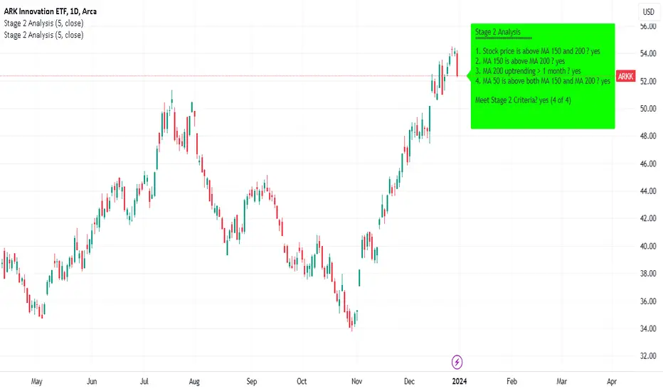
[KVA]Body Percentage Counter This indicator presents a comprehensive view of the historical candle data within user-defined body percentage ranges. Each column represents a specific body size percentage threshold, starting from as low as 0.01% and extending up to 20%.
The rows categorize candles by their closing and opening price differences, effectively sorting them into green (bullish) and red (bearish) candles based on whether they closed higher or lower than their opening prices.
First Row of the table is the bu
For developers, this table can be immensely useful in determining stop-loss ranges. By analyzing the frequency of candles that fall within certain body percentage ranges, developers can better understand where to set stop-loss orders. For instance, if a developer notices a high frequency of candles with body sizes within a specific percentage range, they may choose to set their stop-loss orders outside of this range to avoid being stopped out by normal market fluctuations.
Moreover, the indicator can be used to:
Volatility Assessment : The indicator can be used to gauge market volatility. Smaller bodies may indicate consolidation periods, while larger bodies might suggest more volatile market conditions.
Optimize Trading Strategies : Adjust entry and exit points based on the prevalence of certain candle sizes.
Risk Management : Determine the commonality of price movements within a certain range to better manage risks.
Backtesting : Use historical data to backtest how different stop-loss ranges would have performed in the past.
Comparative Analysis : Traders can compare the frequency of different body sizes over a selected period, providing insights into how the market is evolving.
Educational Use : For new traders, the indicator can serve as an educational tool to understand the implications of candlestick sizes and their relationship with market dynamics
The data provided in this output can guide developers to make more informed decisions about where to place stop-loss orders, potentially increasing the effectiveness of their trading algorithms or manual trading strategies.
The output of the " Body Percentage Counter" indicator is organized into a table format, which can be broken down as follows:
Header (First Row) : This row lists the body percentage thresholds used to categorize the candles. It starts from 0.01% and increases incrementally to 20%. These thresholds are likely set by the user and represent the range of candle body sizes as a percentage of the total candle size.
Green Candle Count (Second Row) : This row displays the count of green candles—candles where the close price is higher than the open price—that fall within each body percentage threshold. For example, under the column "0.01", the number 25 indicates there are 25 green candles whose body size is 0.01% of the total candle size.
Red Candle Count (Third Row) : This row shows the count of red candles—candles where the close price is lower than the open price—for each body percentage threshold. The numbers in this row reflect the number of red candles that match the body percentage criteria in the corresponding column.
Total Candle Count (Fourth Row) : This row sums the counts of both green and red candles for each body percentage threshold, providing a total count of candles that have a body size within the specific range. For instance, if under "0.01" the green count is 25 and the red count is 26, then the total would be 51.
This organized data representation allows users to quickly assess the distribution of candle body sizes over a historical period, which is especially useful for determining the frequency of price movements that are significant enough to consider for stop-loss settings or other trade management decisions.
CCI+EMA Strategy with Percentage or ATR TP/SL [Alifer]This is a momentum strategy based on the Commodity Channel Index (CCI), with the aim of entering long trades in oversold conditions and short trades in overbought conditions.
Optionally, you can enable an Exponential Moving Average (EMA) to only allow trading in the direction of the larger trend. Please note that the strategy will not plot the EMA. If you want, for visual confirmation, you can add to the chart an Exponential Moving Average as a second indicator, with the same settings used in the strategy’s built-in EMA.
The strategy also allows you to set internal Stop Loss and Take Profit levels, with the option to choose between Percentage-based TP/SL or ATR-based TP/SL.
The strategy can be adapted to multiple assets and timeframes:
Pick an asset and a timeframe
Zoom back as far as possible to identify meaningful positive and negative peaks of the CCI
Set Overbought and Oversold at a rough average of the peaks you identified
Adjust TP/SL according to your risk management strategy
Like the strategy? Give it a boost!
Have any questions? Leave a comment or drop me a message.
CAUTIONARY WARNING
Please note that this is a complex trading strategy that involves several inputs and conditions. Before using it in live trading, it is highly recommended to thoroughly test it on historical data and use risk management techniques to safeguard your capital. After backtesting, it's also highly recommended to perform a first live test with a small amount. Additionally, it's essential to have a good understanding of the strategy's behavior and potential risks. Only risk what you can afford to lose .
USED INDICATORS
1 — COMMODITY CHANNEL INDEX (CCI)
The Commodity Channel Index (CCI) is a technical analysis indicator used to measure the momentum of an asset. It was developed by Donald Lambert and first published in Commodities magazine (now Futures) in 1980. Despite its name, the CCI can be used in any market and is not just for commodities. The CCI compares current price to average price over a specific time period. The indicator fluctuates above or below zero, moving into positive or negative territory. While most values, approximately 75%, fall between -100 and +100, about 25% of the values fall outside this range, indicating a lot of weakness or strength in the price movement.
The CCI was originally developed to spot long-term trend changes but has been adapted by traders for use on all markets or timeframes. Trading with multiple timeframes provides more buy or sell signals for active traders. Traders often use the CCI on the longer-term chart to establish the dominant trend and on the shorter-term chart to isolate pullbacks and generate trade signals.
CCI is calculated with the following formula:
(Typical Price - Simple Moving Average) / (0.015 x Mean Deviation)
Some trading strategies based on CCI can produce multiple false signals or losing trades when conditions turn choppy. Implementing a stop-loss strategy can help cap risk, and testing the CCI strategy for profitability on your market and timeframe is a worthy first step before initiating trades.
2 — AVERAGE TRUE RANGE (ATR)
The Average True Range (ATR) is a technical analysis indicator that measures market volatility by calculating the average range of price movements in a financial asset over a specific period of time. The ATR was developed by J. Welles Wilder Jr. and introduced in his book “New Concepts in Technical Trading Systems” in 1978.
The ATR is calculated by taking the average of the true range over a specified period. The true range is the greatest of the following:
The difference between the current high and the current low.
The difference between the previous close and the current high.
The difference between the previous close and the current low.
The ATR can be used to set stop-loss orders. One way to use ATR for stop-loss orders is to multiply the ATR by a factor (such as 2 or 3) and subtract it from the entry price for long positions or add it to the entry price for short positions. This can help traders set stop-loss orders that are more adaptive to market volatility.
3 — EXPONENTIAL MOVING AVERAGE (EMA)
The Exponential Moving Average (EMA) is a type of moving average (MA) that places a greater weight and significance on the most recent data points.
The EMA is calculated by taking the average of the true range over a specified period. The true range is the greatest of the following:
The difference between the current high and the current low.
The difference between the previous close and the current high.
The difference between the previous close and the current low.
The EMA can be used by traders to produce buy and sell signals based on crossovers and divergences from the historical average. Traders often use several different EMA lengths, such as 10-day, 50-day, and 200-day moving averages.
The formula for calculating EMA is as follows:
Compute the Simple Moving Average (SMA).
Calculate the multiplier for weighting the EMA.
Calculate the current EMA using the following formula:
EMA = Closing price x multiplier + EMA (previous day) x (1-multiplier)
STRATEGY EXPLANATION
1 — INPUTS AND PARAMETERS
The strategy uses the Commodity Channel Index (CCI) with additional options for an Exponential Moving Average (EMA), Take Profit (TP) and Stop Loss (SL).
length : The period length for the CCI calculation.
overbought : The overbought level for the CCI. When CCI crosses above this level, it may signal a potential short entry.
oversold : The oversold level for the CCI. When CCI crosses below this level, it may signal a potential long entry.
useEMA : A boolean input to enable or disable the use of Exponential Moving Average (EMA) as a filter for long and short entries.
emaLength : The period length for the EMA if it is used.
2 — CCI CALCULATION
The CCI indicator is calculated using the following formula:
(src - ma) / (0.015 * ta.dev(src, length))
src is the typical price (average of high, low, and close) and ma is the Simple Moving Average (SMA) of src over the specified length.
3 — EMA CALCULATION
If the useEMA option is enabled, an EMA is calculated with the given emaLength .
4 — TAKE PROFIT AND STOP LOSS METHODS
The strategy offers two methods for TP and SL calculations: percentage-based and ATR-based.
tpSlMethod_percentage : A boolean input to choose the percentage-based method.
tpSlMethod_atr : A boolean input to choose the ATR-based method.
5 — PERCENTAGE-BASED TP AND SL
If tpSlMethod_percentage is chosen, the strategy calculates the TP and SL levels based on a percentage of the average entry price.
tp_percentage : The percentage value for Take Profit.
sl_percentage : The percentage value for Stop Loss.
6 — ATR-BASED TP AND SL
If tpSlMethod_atr is chosen, the strategy calculates the TP and SL levels based on Average True Range (ATR).
atrLength : The period length for the ATR calculation.
atrMultiplier : A multiplier applied to the ATR to set the SL level.
riskRewardRatio : The risk-reward ratio used to calculate the TP level.
7 — ENTRY CONDITIONS
The strategy defines two conditions for entering long and short positions based on CCI and, optionally, EMA.
Long Entry: CCI crosses below the oversold level, and if useEMA is enabled, the closing price should be above the EMA.
Short Entry: CCI crosses above the overbought level, and if useEMA is enabled, the closing price should be below the EMA.
8 — TP AND SL LEVELS
The strategy calculates the TP and SL levels based on the chosen method and updates them dynamically.
For the percentage-based method, the TP and SL levels are calculated as a percentage of the average entry price.
For the ATR-based method, the TP and SL levels are calculated using the ATR value and the specified multipliers.
9 — EXIT CONDITIONS
The strategy defines exit conditions for both long and short positions.
If there is a long position, it will be closed either at TP or SL levels based on the chosen method.
If there is a short position, it will be closed either at TP or SL levels based on the chosen method.
Additionally, positions will be closed if CCI crosses back above oversold in long positions or below overbought in short positions.
10 — PLOTTING
The script plots the CCI line along with overbought and oversold levels as horizontal lines.
The CCI line is colored red when above the overbought level, green when below the oversold level, and white otherwise.
The shaded region between the overbought and oversold levels is plotted as well.
WebhookJsonMsgLibrary "WebhookJsonMsg"
This webhook json message library provides convenient functions for building JSON messages
Used to manage automatic transaction orders and positions
method buildWebhookJson(msg)
Builds the final JSON payload from a WebhookMessage type.
Namespace types: WebhookMessage
Parameters:
msg (WebhookMessage)
Returns: A JSON Payload.
Dict
Define some constant values
Fields:
OPEN_LONG (series string)
OPEN_SHORT (series string)
CLOSE_LONG (series string)
CLOSE_SHORT (series string)
LIMIT (series string)
MARKET (series string)
U_MARGIN (series string)
C_MARGIN (series string)
SPOT (series string)
WebhookMessage
Webhook message structure.
Fields:
strategyId (series string)
signalNo (series string)
symbol (series string)
symbolType (series string)
orderSide (series string)
price (series string)
orderType (series string)
takeProfitPrice (series string)
stopLossPrice (series string)
timestamp (series string)
accessKey (series string)

Sushi Trend [HG]🍣 The Sushi Roll, a trading concept conceived at a restaurant by Mark Fisher.
While the indicator itself goes by Sushi Trend, it is completely backed by the idea of Mark Fisher's Sushi Roll Reversal Pattern. No, it has nothing to do with raw fish, it just so happens that somebody was ordering sushi during the discussion of the idea, and that's how it got its name.
📝 Origin
First mentioned in his book, The Logical Trader --- the idea of the Sushi Roll is to serve as an early warning system to identify reversals in the market. Fisher defines the pattern as a series of 10 bars, split into two different sections, seen as 5 and 5. In order for the pattern to be emitted, the 5 bars to the right must completely engulf the 5 bars to the left. It's not a super complex system and is in fact extremely simple to grasp.
📈 Supertrend Similarities
Instead of displaying the pattern in the way Fisher meant for it to be portrayed (as seen in the photo above), I instead turned it into an indicator similar to that of Supertrend while also inheriting the same concepts from the pattern. I did this because the pattern itself has inconsistencies which can be quite noticeable when trading with it after a while. For example, these patterns can occur even during consolidating periods, and even though the pattern is meant to be recognized during trending markets, the engulfing bars can sometimes be left with indecisive directions.
➡️ The Result
Here is the result, visualized to be better in a trending format. (The indicator will not contain the boxes.)
While Fisher does mention the pattern to include 10 bars, you can actually use this pattern with any number of bars. At the end of the day, it's a concept derived from a discussion at a Japanese restaurant, and a pattern that has been around for years that has seen results. Due to this, I added an input option to control the series of bars for right-bar engulf detection.
To reassure the meaning of the pattern --> "A series of 10 bars" means 5 left bars and 5 right bars. So if you want to check if 5 right bars are engulfing the previous 5 bars (as seen in the photo above), you would want to select 5 in the input settings.
You can learn more about it from the following links
Market Reversals and the Sushi Roll Technique
The Logical Trader