BE-Indicator Aggregator toolkit█ Overview:
BE-Indicator Aggregator toolkit is a toolkit which is built for those we rely on taking multi-confirmation from different indicators available with the traders. This Toolkit aid's traders in understanding their custom logic for their trade setups and provides the summarized results on how it performed over the past.
█ How It Works:
Load the external indicator plots in the indicator input setting
Provide your custom logic for the trade setup
Set your expected SL & TP values
█ Legends, Definitions & Logic Building Rules:
Building the logic for your trade setup plays a pivotal role in the toolkit, it shall be broken into parts and toolkit aims to understand each of the logical parts of your setup and interpret the outcome as trade accuracy.
Toolkit broadly aims to understand 4 types of inputs in "Condition Builder"
Comments : Line which starts with single quotation ( ' ) shall be ignored by toolkit while understanding the logic.
Note: Blank line space or less than 3 characters are treated equally to comments.
Long Condition: Line which starts with " L- " shall be considered for identifying Long setups.
Short Condition: Line which starts with " S- " shall be considered for identifying Short setups.
Variables: Line which starts with " VAR- " shall be considered as variables. Variables can be one such criteria for Long or short condition.
Building Rules: Define all variables first then specify the condition. The usual declare and assign concept of programming. :p)
Criteria Rules: Criteria are individual logic for your one parent condition. multiple criteria can be present in one condition. Each parameter should be delimited with ' | ' key and each criteria should be delimited with ' , ' (Comma with a space - IMPORTANT!!!)
█ Sample Codes for Conditional Builder:
For Trading Long when Open = Low
For Trading Short when Open = High with a Red candle
'Long Setup <---- Comment
L-O|E|L
' E <- in the above line refers to Equals ' = '
'Short Setup
S-AND:O|E|H, O|G|C
' 2 Criteria for used building one condition. Since, both have to satisfied used "AND:" logic.
Understanding of Operator Legends:
"E" => Refers to Equals
"NE" => Refers to Not Equals
"NEOR" => Logical value is Either Comparing value 1 or Comparing value 2
"NEAND" => Logical value is Comparing value 1 And Comparing value 2
"G" => Logical value Greater than Comparing value 1
"GE" => Logical value Greater than and equal to Comparing value 1
"L" => Logical value Lesser than Comparing value 1
"LE" => Logical value Lesser than and equal to Comparing value 1
"B" => Logical value is Between Comparing value 1 & Comparing value 2
"BE" => Logical value is Between or Equal to Comparing value 1 & Comparing value 2
"OSE" => Logical value is Outside of Comparing value 1 & Comparing value 2
"OSI" => Logical value is Outside or Equal to Comparing value 1 & Comparing value 2
"ERR" => Logical value is 'na'
"NERR" => Logical value is not 'na'
"CO" => Logical value Crossed Over Comparing value 1
"CU" => Logical value Crossed Under Comparing value 1
Understanding of Condition Legends:
AND: -> All criteria's to be satisfied for the condition to be True.
NAND: -> Output of AND condition shall be Inversed for the condition to be True.
OR: -> One of criteria to be satisfied for the condition to be True.
NOR: -> Output of OR condition shall be Inversed for the condition to be True.
ATLEAST:X: -> At-least X no of criteria to be satisfied for the condition to be True.
Note: "X" can be any number
NATLEAST:X: -> Output of ATLEAST condition shall be Inversed for the condition to be True
WASTRUE:X: -> Single criteria WAS TRUE within X bar in past for the condition to be True.
Note: "X" can be any number.
ISTRUE:X: -> Single criteria is TRUE since X bar in past for the condition to be True.
Note: "X" can be any number.
Understanding of Variable Legends:
While Condition Supports 8 Types, Variable supports only 6 Types listed below
AND: -> All criteria's to be satisfied for the Variable to be True.
NAND: -> Output of AND condition shall be Inversed for the Variable to be True.
OR: -> One of criteria to be satisfied for the Variable to be True.
NOR: -> Output of OR condition shall be Inversed for the Variable to be True.
ATLEAST:X: -> At-least X no of criteria to be satisfied for the Variable to be True.
Note: "X" can be any number
NATLEAST:X: -> Output of ATLEAST condition shall be Inversed for the Variable to be True
█ Sample Outputs with Logics:
1. RSI Indicator + Technical Indicator: StopLoss: 2.25 against Reward ratio of 1.75 (3.94 value)
Plots Used in Indicator Settings:
Source 1:- RSI
Source 2:- RSI Based MA
Source 3:- Strong Buy
Source 4:- Strong Sell
Logic Used:
For Long Setup : RSI Should be above RSI Based MA, RSI has been Rising when compared to 3 candles ago, Technical Indicator signaled for a Strong Buy on the current candle, however in last 6 candles Technical indicator signaled for Strong Sell.
Similarly Inverse for Short Setup.
L-AND:ES1|GE|ES2, ES1|G|ES1
L-ES3|E|1
L-OR:ES4 |E|1, ES4 |E|1, ES4 |E|1, ES4 |E|1, ES4 |E|1, ES4 |E|1
S-AND:ES1|LE|ES2, ES1|L|ES1
S-ES4|E|1
S-OR:ES3 |E|1, ES3 |E|1, ES3 |E|1, ES3 |E|1, ES3 |E|1, ES3 |E|1
'Note: Last OR condition can also be written by using WASTRUE definition like below
'L-WASTRUE:6:ES4|E|1
'S-WASTRUE:6:ES3|E|1
Output:
2. Volumatic Support / Resistance Levels :
Plots Used in Indicator Settings:
Source 1:- Resistance
Source 2:- Support
Logic Used:
For Long Setup : Long Trade on Liquidity Support.
For Short Setup : Short Trade on Liquidity Resistance.
'Variable Named "ChkLowTradingAbvSupport" is declared to check if last 3 candles is trading above support line of liquidity.
VAR-ChkLowTradingAbvSupport:AND:L|G|ES2, L |G|ES2, L |G|ES2
'Variable Named "ChkCurBarClsdAbv4thBarHigh" is declared to check if current bar closed above the high of previous candle where the Liquidity support is taken (4th Bar).
VAR-ChkCurBarClsdAbv4thBarHigh:OR:C|GE|H , L|G|H
'Combining Condition and Variable to Initiate Long Trade Logic
L-L |LE|ES2
L-AND:ChkLowTradingAbvSupport, ChkCurBarClsdAbv4thBarHigh
VAR-ChkHghTradingBlwRes:AND:H|L|ES1, H |L|ES1, H |L|ES1
VAR-ChkCurBarClsdBlw4thBarLow:OR:C|LE|L , H|L|L
S-H |GE|ES1
S-AND:ChkHghTradingBlwRes, ChkCurBarClsdBlw4thBarLow
Output 1: Day Trading Version
Output 2: Scalper Version
Output 3: Position Version
스크립트에서 "liquidity"에 대해 찾기

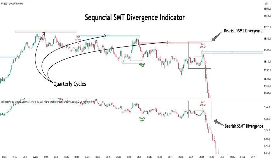
Quarterly Theory ICT 04 [TradingFinder] SSMT 4Quarter Divergence🔵 Introduction
Sequential SMT Divergence is an advanced price-action-based analytical technique rooted in the ICT (Inner Circle Trader) methodology. Its primary objective is to identify early-stage divergences between correlated assets within precise time structures. This tool not only breaks down market structure but also enables traders to detect engineered liquidity traps before the market reacts.
In simple terms, SMT (Smart Money Technique) occurs when two correlated assets—such as indices (ES and NQ), currency pairs (EURUSD and GBPUSD), or commodities (Gold and Silver)—exhibit different reactions at key price levels (swing highs or lows). This lack of alignment is often a sign of smart money manipulation and signals a lack of confirmation in the ongoing trend—hinting at an imminent reversal or at least a pause in momentum.
In its Sequential form, SMT divergences are examined through a more granular temporal lens—between intraday quarters (Q1 through Q4). When SMT appears at the transition from one quarter to another (e.g., Q1 to Q2 or Q3 to Q4), the signal becomes significantly more powerful, often aligning with a critical phase in the Quarterly Theory—a framework that segments market behavior into four distinct phases: Accumulation, Manipulation, Distribution, and Reversal/Continuation.
For instance, a Bullish SMT forms when one asset prints a new low while its correlated counterpart fails to break the corresponding low from the previous quarter. This usually indicates absorption of selling pressure and the beginning of accumulation by smart money. Conversely, a Bearish SMT arises when one asset makes a higher high, but the second asset fails to confirm, signaling distribution or a fake-out before a decline.
However, SMT alone is not enough. To confirm a true Market Structure Break (MSB), the appearance of a Precision Swing Point (PSP) is essential—a specific candlestick formation on a lower timeframe (typically 5 to 15 minutes) that reveals the entry of institutional participants. The combination of SMT and PSP provides a more accurate entry point and better understanding of premium and discount zones.
The Sequential SMT Indicator, introduced in this article, dynamically scans charts for such divergence patterns across multiple sessions. It is applicable to various markets including Forex, crypto, commodities, and indices, and shows particularly strong performance during mid-week sessions (Wednesdays and Thursdays)—when most weekly highs and lows tend to form.
Bullish Sequential SMT :
Bearish Sequential SMT :
🔵 How to Use
The Sequential SMT (SSMT) indicator is designed to detect time and structure-based divergences between two correlated assets. This divergence occurs when both assets print a similar swing (high or low) in the previous quarter (e.g., Q3), but in the current quarter (e.g., Q4), only one asset manages to break that swing level—while the other fails to reach it.
This temporal mismatch is precisely identified by the SSMT indicator and often signals smart money activity, a market phase transition, or even the presence of an engineered liquidity trap. The signal becomes especially powerful when paired with a Precision Swing Point (PSP)—a confirming candle on lower timeframes (5m–15m) that typically indicates a market structure break (MSB) and the entry of smart liquidity.
🟣 Bullish Sequential SMT
In the previous quarter, both assets form a similar swing low.
In the current quarter, one asset (e.g., EURUSD) breaks that low and trades below it.
The other asset (e.g., GBPUSD) fails to reach the same low, preserving the structure.
This time-based divergence reflects declining selling pressure, potential absorption, and often marks the end of a manipulation phase and the start of accumulation. If confirmed by a bullish PSP candle, it offers a strong long opportunity, with stop-losses defined just below the swing low.
🟣 Bearish Sequential SMT
In the previous quarter, both assets form a similar swing high.
In the current quarter, one asset (e.g., NQ) breaks above that high.
The other asset (e.g., ES) fails to reach that high, remaining below it.
This type of divergence signals weakening bullish momentum and the likelihood of distribution or a fake-out before a price drop. When followed by a bearish PSP candle, it sets up a strong shorting opportunity with targets in the discount zone and protective stops placed above the swing high.
🔵 Settings
⚙️ Logical Settings
Quarterly Cycles Type : Select the time segmentation method for SMT analysis.
Available modes include: Yearly, Monthly, Weekly, Daily, 90 Minute, and Micro.
These define how the indicator divides market time into Q1–Q4 cycles.
Symbol : Choose the secondary asset to compare with the main chart asset (e.g., XAUUSD, US100, GBPUSD).
Pivot Period : Sets the sensitivity of the pivot detection algorithm. A smaller value increases responsiveness to price swings.
Activate Max Pivot Back : When enabled, limits the maximum number of past pivots to be considered for divergence detection.
Max Pivot Back Length : Defines how many past pivots can be used (if the above toggle is active).
Pivot Sync Threshold : The maximum allowed difference (in bars) between pivots of the two assets for them to be compared.
Validity Pivot Length : Defines the time window (in bars) during which a divergence remains valid before it's considered outdated.
🎨 Display Settings
Show Cycle :Toggles the visual display of the current Quarter (Q1 to Q4) based on the selected time segmentation
Show Cycle Label : Shows the name (e.g., "Q2") of each detected Quarter on the chart.
Show Bullish SMT Line : Draws a line connecting the bullish divergence points.
Show Bullish SMT Label : Displays a label on the chart when a bullish divergence is detected.
Bullish Color : Sets the color for bullish SMT markers (label, shape, and line).
Show Bearish SMT Line : Draws a line for bearish divergence.
Show Bearish SMT Label : Displays a label when a bearish SMT divergence is found.
Bearish Color : Sets the color for bearish SMT visual elements.
🔔 Alert Settings
Alert Name : Custom name for the alert messages (used in TradingView’s alert system).
Message Frequency :
All: Every signal triggers an alert.
Once Per Bar: Alerts once per bar regardless of how many signals occur.
Per Bar Close: Only triggers when the bar closes and the signal still exists.
Time Zone Display : Choose the time zone in which alert timestamps are displayed (e.g., UTC).
Bullish SMT Divergence Alert : Enable/disable alerts specifically for bullish signals.
Bearish SMT Divergence Alert : Enable/disable alerts specifically for bearish signals
🔵 Conclusion
The Sequential SMT (SSMT) indicator is a powerful and precise tool for identifying structural divergences between correlated assets within a time-based framework. Unlike traditional divergence models that rely solely on sequential pivot comparisons, SSMT leverages Quarterly Theory, in combination with concepts like liquidity sweeps, market structure breaks (MSB) and precision swing points (PSP), to provide a deeper and more actionable view of market dynamics.
By using SSMT, traders gain not only the ability to identify where divergence occurs, but also when it matters most within the market cycle. This empowers them to anticipate major moves or traps before they fully materialize, and position themselves accordingly in high-probability trade zones.
Whether you're trading Forex, crypto, indices, or commodities, the true strength of this indicator is revealed when used in sync with the Accumulation, Manipulation, Distribution, and Reversal phases of the market. Integrated with other confluence tools and market models, SSMT can serve as a core component in a professional, rule-based, and highly personalized trading strategy.
Flat Tops/Bottoms aka Devil's MarkThis Pine script indicator is designed to visually depict price inefficiencies, as identified by Flat Top/Bottom Candles (aka Devil's Mark). A Flat Top/Bottom Candle is a scenario where there is an absence of a wick at the top or the bottom of the candle. These represent zones of inefficiency and will frequently act as magnets for price that the market will strive to rebalance in accordance with ICT principles.
Relevance:
Flat Top/Bottom Candles are zones where price delivery didn't provide opportunity for manipulation representing an inefficiency that the market will seek to rebalance. Consequently, these zones can provide good targets for entries in the opposite direction or take profit targets for previous entries in the direction of the Flat Top/Bottom Candle.
How It Works:
The indicator keeps track of all Flat Top/Bottom Candles from the beginning of the available history. It automatically removes all mitigated Flat Top/Bottom Candles, which are situations where the price has gone past the candle without a wick.
Configurability:
You can configure the colors, style & width of the lines used to represent flat top/bottom candles.
What makes this indicator different:
Designed with high performance in mind, to reduce impact on chart render time.
Only keeping the currently valid flat top/bottoms on the chart.

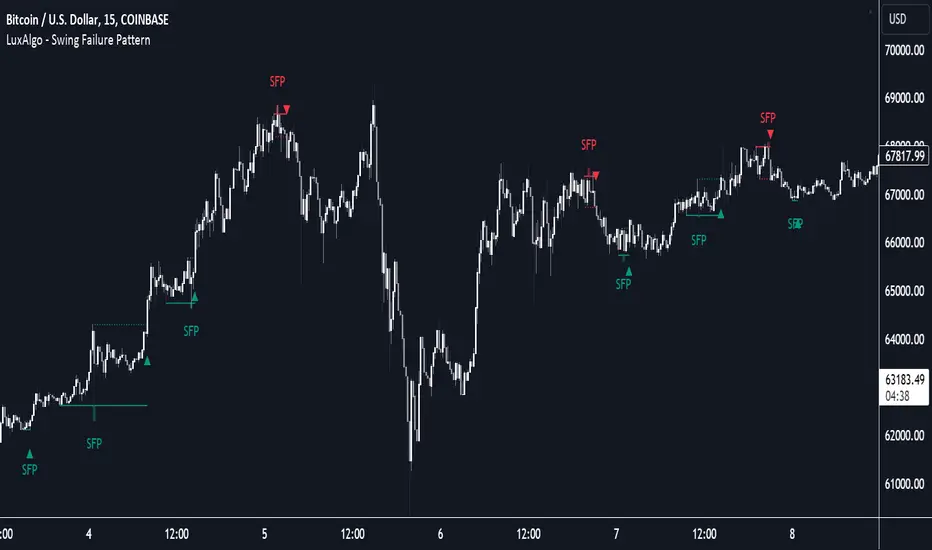
Swing Failure Pattern (SFP) [LuxAlgo]The Swing Failure Pattern indicator highlights Swing Failure Patterns (SFP) on the user chart, a pattern occurring during liquidity generation from significant market participants.
A Confirmation level used to confirm a trend reversal is also included. Users can additionally filter out SFP based on a set Volume % Threshold .
🔶 USAGE
Swing failure patterns occur when candle wicks exceed (above/below) a recent swing level but close back below/above it, and occur from more significant market participants engineering liquidity. This pattern can be indicative of a potential trend reversal.
A label and an accentuated wick line highlight the SFP (both can be disabled).
Using a higher "Swings" period will not return different SFP but will however potentially reduce their detection rate.
🔹 Confirmation Level
The confirmation level is the highest point between the previous swing and SFP for a bullish SFP, and the lowest point for a bearish SFP. This level allows confirming a trend reversal after an SFP once the price breaks it.
A small triangle will be displayed when the price closes beyond the confirmation level.
A more reactive and contrarian approach could use the SFP as an entry point, and the confirmation level for taking (partial) profit, or stop loss. The example below shows a possible scenario:
🔹 Volume % Threshold
During the occurrence of an SFP, the Volume % Threshold option allows comparing the cumulative volume outside the Swing level to the total volume of the candle. The following options are included:
Volume outside swing < Threshold: Volume outside the Swing level needs to be lower than x % of total candle volume. Prevent excessive liquidity generation.
Volume outside swing > Threshold: Volume outside the Swing level needs to be higher than x % of total candle volume. Requires more significant liquidity to be generated.
None: No extra filter is applied
Note that in the above case, the left SFP is no longer highlighted because the volume above the swing level was higher than the 25% threshold of the total volume.
When we change the setting to "Volume outside swing > Threshold", we get the reversed situation.
The "Volume outside Swing level" is obtained using intrabar - Lower TimeFrame (LTF) data.
At the intrabar (LTF) level, there are a maximum of 100K bars available. When using the Volume % Threshold filter, a vertical line will highlight the maximum period during which intrabars are available.
🔶 DETAILS
🔹 LTF Settings
When 'Auto' is enabled (Settings, LTF), the LTF will be the nearest possible x times smaller TF than the current TF. When 'Premium' is disabled, the minimum TF will always be 1 minute to ensure TradingView plans lower than Premium don't get an error.
Examples with current Daily TF (when Premium is enabled):
500 : 3-minute LTF
1500 (default): 1-minute LTF
5000: 30 seconds LTF (1 minute if Premium is disabled)
The concerning LTF can be seen at the right-top (default) corner.
🔶 SETTINGS
Swings: Period used for the swing detection, with higher values returning longer-term Swing Levels.
Bullish SFP: enable/disable bullish Swing Failure Patterns.
Bearish SFP: enable/disable bearish Swing Failure Patterns.
🔹 Volume Validation
Validation:
Volume outside swing < Threshold: The volume outside the swing level needs to be lower than x % of the total volume.
Volume outside swing > Threshold: The volume outside the swing level needs to be higher than x % of the total volume.
None: No extra validation is applied.
Volume % Threshold: % of total volume as threshold.
Auto + multiple: Adjusts the initial set LTF
LTF: LTF setting
Premium: Enable when your TradingView plan is Premium or higher
🔹 Dashboard
Show Dashboard: Display applied Lower Timeframe (LTF)
Location: Location of the dashboard
Size: Size of the dashboard
🔹 Style
Swing Lines
Confirmation Lines
Swing Failure Wick
Swing Failure Label
Lines / Labels: Color for lines and labels
SFP Wicks: Color for SFP wick line
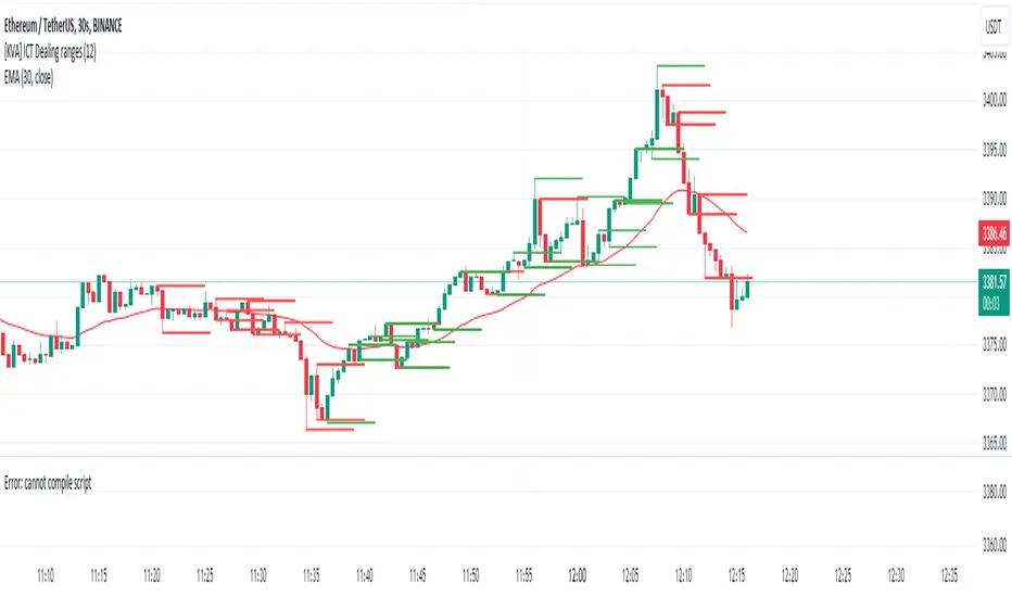
[KVA] ICT Dealing rangesNaive aproach of Dynamic Detection of Dealing Ranges:
The script dynamically identifies dealing ranges based on sequences of upward or downward price movements. It uses arrays to track the highest highs and lowest lows after detecting two consecutive up or down bars, a fundamental step towards understanding market structure and potential shifts in momentum.
ICT Concept: Order Blocks & Fair Value Gaps. This aspect can be linked to the identification of order blocks (bullish or bearish) and fair value gaps. Order blocks are essentially the last bearish or bullish candle before a significant price move, which this script could approximate by identifying the highs and lows of potential reversal zones.
Red and Green Ranges for Bullish and Bearish Movements:
The script separates these movements into red (bearish) and green (bullish) ranges, effectively categorizing potential areas of selling and buying pressure.
ICT Concept: Liquidity Pools. Red ranges could be indicative of areas where selling might occur, potentially leading to liquidity pools below these ranges. Conversely, green ranges might indicate potential buying pressure, with liquidity pools above. These areas are critical for ICT traders, as they often represent zones where price may return to "hunt" for liquidity.
Horizontal Lines for High and Low Points:
The indicator draws horizontal lines at the high and low points of these ranges, offering visual cues for significant levels.
ICT Concept: Breaker Blocks & Mitigation Sequences. The high and low points of these ranges can be seen as potential breaker blocks or areas for future mitigation sequences. In ICT terms, breaker blocks are areas where institutional orders have overwhelmed retail stop clusters, creating potential entry points for trend continuation or reversal. The high and low points marked by the indicator could serve as references for these sequences, where price might return to retest these levels.
Customizability and Historical Depth:
With inputs like rangePlot and maxBarsBack, the indicator allows for customization of the number of ranges to display and how far back in the chart history it looks to identify these ranges. This flexibility is crucial for tailoring the analysis to different trading strategies and timeframes.
ICT Concept: Market Structure Analysis. The ability to adjust the depth and number of ranges plotted caters to a detailed market structure analysis, an essential component of ICT methodology. Traders can adjust these parameters to better understand the distribution of buying and selling pressure over time and how actions have shaped price movements.
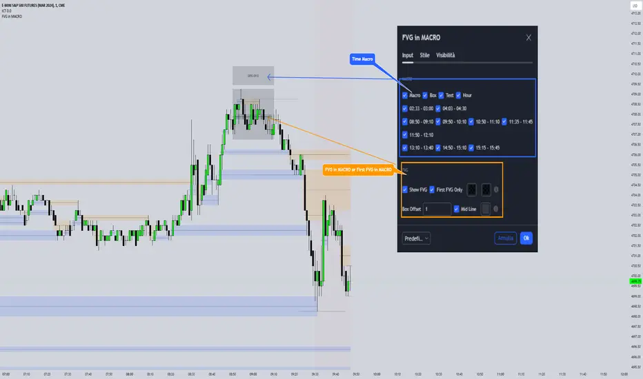
FVG in MACROGuided by ICT tutoring, I created this versatile indicator to scan the FVG in MACRO time.
This indicator combines the MACRO time with the Fair value GAP (FVG) in an alternative way, showing a simple way of viewing the FVG within the MACRO time, so you can have a clearer view of which direction the MACRO is influencing
''MACRO is a delivery time frame of the interbank price in which it undergoes a series of controls and is likely to move towards liquidity.''
The user has the possibility to:
- Choose the relevant MACRO time
- Choose whether to view all FVGs in the MACROS
- Choose to view only the First FVG at each MACRO
The indicator should be used as shown by the ICT in its concepts, during the MACRO time the price can consolidate or can head towards liquidity.
The probability that the direction is correct increases with respect for the FVG, in this way it is possible to evaluate the entry zone in the FVG and the Take profit zone for Liquidity
As in the following example:
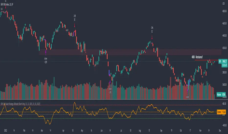
Fair Value Strategy - ekmllThis is a strategy using SPX's Fair Value derived from Net Liquidity.
The main difference between this one and calebsandfort's one is net liquidity values in this one are calculated in TradingView and doesn't need author's daily library updates to function.
Net Liquidity function is simply: Fed Balance Sheet - Treasury General Account - Reverse Repo Balance
Formula for calculating the fair value of and Index using Net Liquidity looks like this: (WALCL - WTREGEN - RRPONTSYD)/1000000000/scalar - subtractor
The Index Fair Value is then subtracted from the Index value which creates an oscillating diff value.
When diff is greater than the overbought threshold, Index is considered overbought and we go short/sell.
When diff is less than the oversold signal, Index is considered oversold and we cover/buy.
Parameters:
Index: SPX, NDX, RUT
Strategy: Short Only, Long Only, Long/Short
Inverse (bool): check if using an inverse ETF to go long instead of short.
Scalar (float)
Subtractor (int)
Overbought Threshold (int)
Oversold Threshold (int)
Start After Date: When the strategy should start trading
Close Date: Day to close open trades. I just like it to get complete results rather than the strategy ending with open trades.
I've optimized the parameters for SPX.

Fair Value Strategy UltimateThis is a strategy using an index's (SPX, NDX, RUT) Fair Value derived from Net Liquidity.
Net Liquidity function is simply: Fed Balance Sheet - Treasury General Account - Reverse Repo Balance
Formula for calculating the fair value of and Index using Net Liquidity looks like this: net_liquidity/1000000000/scalar - subtractor
The Index Fair Value is then subtracted from the Index value which creates an oscillating diff value.
When diff is greater than the overbought threshold, Index is considered overbought and we go short/sell.
When diff is less than the oversold signal, Index is considered oversold and we cover/buy.
The net liquidity values I calculate outside of TradingView. If you'd like the strategy to work for future dates, you'll need to update the reference to my NetLiquidityLibrary , which I update daily.
Parameters:
Index: SPX, NDX, RUT
Strategy: Short Only, Long Only, Long/Short
Inverse (bool): check if using an inverse ETF to go long instead of short.
Scalar (float)
Subtractor (int)
Overbought Threshold (int)
Oversold Threshold (int)
Start After Date: When the strategy should start trading
Close Date: Day to close open trades. I just like it to get complete results rather than the strategy ending with open trades.
Optimal Parameters:
I've optimized the parameters for each index using the python backtesting library and they are as follows =>
SPX
Scalar: 1.1
Subtractor: 1425
OB Threshold: 0
OS Threshold: -175
NDX
Scalar: 0.5
Subtractor: 250
OB Threshold: 0
OS Threshold: -25
RUT
Scalar: 3.2
Subtractor: 50
OB Threshold: 25
OS Threshold: -25

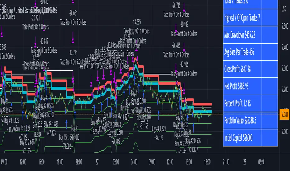
3Commas Bot DCA Backtester & Signals FREEThis is a DCA Strategy backtester + signals, built to emulate the 3Commas DCA bots. It uses your choice of 4 different buy signals, 2 of which can be adjusted in the settings. Everything is customizable so you can backtest specific settings with different buy signals and find the best performing strategy for your risk tolerance and capital. It can be used to backtest strategies on stocks as well, but just make sure your base order is larger than the share price for the entire backtesting range or it will not calculate properly.
You can use this template to code your own buy signals and then backtest them as a DCA strategy if you know some basic pine script.
The indicator shows all of your backtesting orders on the chart. The red line is your take profit level, the blue line is your average price level, the white line is your first order and the green lines are your average down orders. If you enable a stop loss in the settings your stop loss will be shown as an orange line once all of your average down orders have been hit, it will not be set until price has dipped below your covered trading range.
These levels update when things change during backtesting so you can visualize your strategy and how it would perform as well as see if your percentage deviation is large enough to cover dips. When backtesting trades are taken, the chart will show where they were taken(in backtesting) along with info on those trades such as the number each order is, the size of that order and the percentage deviation that order is from the initial buy.
SENDING SIGNALS TO 3COMMAS
Tradingview cannot sync this backtester to 3Commas and with the way alerts are setup for strategies on Tradingview, the best option for you to give signals to your bot would be to use this backtester to figure out what trigger you want to use and then setup that indicator separately to send alerts to your bot. All of the indicators used for signals in this backtester are available for free and can be configured to match this backtester and send alerts to 3Commas for you. Just make sure you set your alerts to once per bar close and don’t use less than a 15 second timeframe because then you could trigger the Tradingview threshold for alerts and get your alerts shut off.
You can also use this backtester with your own buy triggers if you know a little pine script. Just make copy of the script and code in your own buy signals and see how it backtests.
INFO PANEL FOR ANALYZING YOUR STRATEGY
The right hand side of the screen will show an info panel that shows a lot of different information so you can quickly see your bot settings and how it performed right on the screen.
In the top right corner you will see in purple your bot settings. These include your stoploss % if turned on, take profit %, average down order %, average down order % multiplier, volume multiplier, max number of orders allowed and size of your base order.
The top section of the first column “Current Trade” shows these stats: the open trade’s average price, the open trade’s take profit price, the open trade’s PNL, how far price is from your open tarde’s take profit level in percentage, your open position size and number of open orders.
The bottom section of the first column “Overall Performance” shows these stats: total number of trades taken during backtesting range, the largest amount of trades that were open at one time during backtesting, the max drawdown, the average number of bars per trade, gross profit, net profit, percent profit from your initial capital, current portfolio value and your initial capital.
CUSTOMIZABLE OPTIONS TO FIND THE PERFECT STRATEGY
Stoploss On/Off
This will turn your stoploss on or off. By default it is set to off and will not affect anything unless turned on.
Stoploss Percentage
This is the percentage below your final average down order price that will be set as a stoploss to keep your account from going too far in the red on big dips.
Take Profit Percentage - This is the percentage of profit you want the trade to hit before taking profit on your entire DCA trade. This level updates everytime you average down.
Average Down Percentage - This is the percentage that price has to drop from your initial order to initiate your first safety order. If the Average Down Percent Multiplier is set to 1 then this percentage will be the same for every average down order.
Average Down Percentage Multiplier - This multiplies your Average Down Percentage so each safety order needs a larger percentage deviation than the previous one. This keeps your buys closer together at the beginning and further apart when you hit more orders so you can extend your trading range but still be aggressive when price is going sideways.
Volume Multiplier Per New Order - This multiplies the size of each trade based on your base order. If you set it to a 2x multiplier then each average down order will be 2 times the size of the last one. So for example, a $100 base order with a 2x multiplier would have these values for the first 3 average down orders: 200, 400, 800.
Size Of Base Order - This is the size of your first position entry and will be used as a starting point for the volume multiplier. If your base order is $100 then it will buy $100 worth of whatever crypto you are backtesting this on. If you are looking at stock charts, you need to make sure your base order is higher than the share price across the entire backtesting range or it will not perform correctly.
Max Number Of Orders - This is the maximum number of orders the bot can take, including your base order. Adjust this to suit the amount of capital you are willing to allocate to your bot based on how much money it will require to run according to your bot settings.
TIPS ON HOW TO USE FOR BEST RESULTS
If you don’t have a lot of capital to work with, then use longer timeframes with a reasonable take profit percentage so that you don’t need a lot of average down orders. You can also try keeping the volume multiplier close to 1.
You can use the 3Commas dca bot settings page to see how much capital you will need for your strategy if you match it to the settings you have on this indicator. You can also check to see how much of a percentage deviation your bot is covering to make sure you have a reasonable range to trade in and orders to cover big dips. You can also check your coverage by seeing how far down the chart the green lines cover, which are your average down orders.
Make sure the initial capital in the properties tab of the settings has enough to cover all of your orders otherwise you will get unrealistic backtesting results. Also, make sure you leave the order size in the properties tab on contracts so it calculates your trades correctly. The only settings you need to touch in the properties tab is the initial capital. Unless you are trading somewhere that has lower commission fees, then you can change that to match, but leave all the other settings as is for it to function properly.
Increasing the volume multiplier will make your average price and take profit target follow the price action a lot closer as price falls, but it can also lead to having very large orders very quickly once you get into the 1.5-3x multiple range. Try using a high volume multiplier with less safety orders and you will get better results, however you need to have money on the sidelines to add on major dips to keep your bot turning a profit. Be very careful with this as greed and impatience will hurt your overall performance. This bot is meant to make money with lots of small wins so don’t get greedy and make sure you have enough money to cover large dips. If you are being aggressive with your bot, then I recommend only using 25% or less of your portfolio to trade aggressively and then use the smart trade feature on 3commas to add chunks of funds to your trades when price dips below your last safety order. Or if you want it to run without any supervision, then use lower volume multipliers and have lots of safety orders that can cover entire bear markets and still keep buying lower.
It’s a good idea to have some capital on the sidelines that you can add in when price dips quickly. This will help lower your average price and allow your bot to get out in profit quicker. 3Commas bot has a smart trade feature that will allow you to track your average price when adding extra funds and it will automatically update your other orders which is very convenient. Look at the longer timeframes when price dips and only add chunks at major areas where price is very likely to bounce. Or you can be aggressive when trading and add to your position when price dips and is at a likely bounce zone to maximize profits.
Only trade coins that have a good amount of liquidity as the larger your orders get, the harder it will be to sell if there isn’t much liquidity. Also, beware of how large your first order is as it will usually be a market order and can move the market if there is not much liquidity.
Since this bot takes a lot of trades and performs best when taking small profits consistently, you will need to factor in exchange fees. The bot is set to .5% commission(you can change this) on the buy and sell orders as most exchanges charge that amount. Some exchanges offer no fee trading on certain coins so be sure to look around for those so you can keep the commissions and maximize profits.
I strongly encourage you to try out a lot of different setting combinations across multiple different coins and do it across a few months to see how it would have performed under various market conditions. This will help you get a better idea of how much of a percentage deviation you’ll need to be able to cover to keep your bot running and making constant profits. You can also use the deep backtesting feature of the strategy panel to see how it would have done, but just beware that the info panel of the indicator will not reflect deep backtesting results, only the normal backtesting range.
MARKETS
This backtester can be used on any market including crypto, stocks, forex & futures. You just need to make sure your base order is larger than the share price when using this on things besides crypto.
TIMEFRAMES
This backtester can be used on all timeframes.
SPX Fair Value Strategy UltimateThis is a strategy using the SPX Fair Value derived from Net Liquidity.
Net Liquidity function is simply: Fed Balance Sheet - Treasury General Account - Reverse Repo Balance
Formula for calculating the fair value of SPX using Net Liquidity looks like this: net_liquidity/1000000000/1.1 -1625
The SPX Fair Value is then subtracted from the SPX value which creates an oscillating diff value.
When diff is greater than 350, SPX is considered overbought and we go short/sell.
When diff is less than -150, SPX is considered oversold and we cover/buy.
The net liquidity values I calculate outside of TradingView. If you'd like the strategy to work for future dates, you'll need to update them.
Paremeters:
Strategy: Short Only, Long Only, Long/Short
Inverse (bool): check if using an inverse ETF to go long instead of short.
Start After Date: When the strategy should start trading
Close Date: Day to close open trades. I just like it to get complete results rather than the strategy ending with open trades.
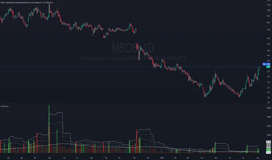
Demand & Supply Zones [eyes20xx]Demand & Supply Zones
This indicator helps to identify large moves driven by institutions.
What qualifies as a zone?
If the price moves (open to close) by more than a certain % in one candle or in a bullish / bearish run of candles, the zone is marked as a Demand or Supply zone .
0.8% is good for Crypto and Forex might be better with 0.4%. Play around with the % to match your requirements.
Active zones
A zone remains active until it is hit by the price. When it becomes inactive, the zone background becomes transparent.
Zone lines
Lines are displayed if the zone is active and within a certain % of the close. 3% is a good setting for Crypto.
A maximum of two lines are displayed for each zone type.

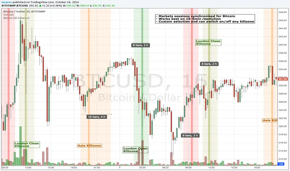
BITCOIN KILL ZONES v2Kill Zones
Kill zones are really liquidity events. Many different market participants often come together and act around these events. The activity itself may be event driven (margin calls or options exercise related activity), portfolio management driven (buy-on-close and asset allocation rebalancing orders) or institutionally driven (larger players needing liquidity to get filled in size) or a combination of any/all three. The point is, this intense cross current of activity at a very specific point in time often occurs near significant technical levels and trends established coming out of these events often persist until the next Kill Zone in approached/entered.
Specifically, there are three Kill Zones and each has its own importance/significance.
1. Asian Kill Zone (1900 - 2300 EST) Considered the "institutional" zone, this zone represents both the launch pad for new trends and also too a reloading area from the post American session. It is the start of a new day (or week) for the world and as such it makes sense this zone will often set the tone for the rest of the world's trading day. Since it is very wide (4 hours) one should pay attention to the Tokyo open (2100 EST) the Beijing open (2120 EST) and the Sydney open (0650 EST previous day).
2. London Kill Zone (0200 - 0400 EST) Considered the center of the financial universe for more than 500 years, Europe still carries a lot of influence within the banking world. Many larger players use the Euro session to establish their positions. As such, the London open often sees the most significant trend establishment activity through any given trading day. Indeed, it has been suggested 80% of all weekly trends are established through Tuesday's London Kill Zone.
3. New York Kill Zone (0830 - 1030 EST) The United States is still by far the world's largest economy and so by default New York's open carries a lot of weight and often comes with a big injection of liquidity. Indeed, most of the world's trade-able assets are priced in US dollars which gives even more significance to political and economic activity within this region. Because it comes relatively late in the globe's trading day, this Kill Zone often sees violent price swings within it's first hour leading to the time tested adage "never trust the first hour of North American trading.
Additional notes:
It has become apparent these Kill Zones are evolving over time and the course of world history. Since the end of the second world war, New York has slowly encroached on London's place as the global center for commercial banking. So much so through the later part of the 20th century New York was considered indeed, the new center of the financial universe. With the end of the cold war that leadership seems to have shifted back toward Europe and away from The United States. Additionally, Japan has slowly lost its former predominance within the global economic landscape while Beijing's has risen dramatically.
Only time will tell how these kill zones will evolve given each region's ever changing political, economic and socioeconomic influences.
Trading Notes:
If you have specific levels of interest odds are the bigger players have the same levels too. If it is indeed a solid level, look for price to trade to your level through the kill zone because the zone is a liquidity event where the bigger players can find enough size to get their big orders filled.
Try to avoid taking positions heading into Kill Zones and look for confirmation of your levels coming out of the event. For the more advanced trader, look to take positions on those level hits through the zone but understand higher time frame players often have far deeper pockets then day traders and can endure far more volatility then us little guys.
Thanks for the contribution to @CRInvestor and @ICT_MHuddleston
VWAP Diario + VWAP 08:00-12:00 ventanas NYWhat it plots
Daily VWAP (main line)
Anchored to the current trading day and only visible between 19:00 and 16:50 New York (UTC-5) to prevent any “ghost” segments.
Dynamic color: turns green when price closes above (bullish bias) and red when price closes below (bearish bias).
Optional standard-deviation/percentage bands (off by default).
08:00–12:00 VWAP (morning line)
Resets at 08:00 NY and shows until 12:00 NY only.
Acts as a morning value guide for early direction and pullbacks.
Clean rendering: Both lines use strict time masks and line breaks, so nothing is drawn outside their windows. You can toggle either line on/off.
How to Read It
Daily VWAP ≈ “fair value” of the whole session; use it for directional bias and confluence.
08:00–12:00 VWAP ≈ “fair value” of the morning; helps refine entries during the open.
Alignment:
Bullish environment: price and 08–12 VWAP sit above the Daily VWAP.
Rotation/mixed: price oscillates between the two lines.
Bearish: price and 08–12 VWAP sit below the Daily VWAP.
Two Mechanical Playbooks
Recommended charts: 1-minute for entries, 5-minute for context on NQ/Nasdaq100.
Primary execution window: 09:30–12:00 NY.
A) Trend Play (Break → Pullback to VWAP)
Goal: Join the day’s impulse with value confirmation.
Rules
Bias filter before 09:30
Bullish: 08–12 VWAP ≥ Daily VWAP; Bearish: 08–12 ≤ Daily.
First push 09:30–09:45 breaks the initial range high (bull) or low (bear).
Entry (pullback into confluence)
Wait for a pullback that tags/wicks the 08–12 VWAP or the Daily VWAP in the direction of bias.
Go long on bullish rejection (close back above); short on bearish rejection.
Stop-loss
Beyond the rejection wick or the touched VWAP (e.g., 1–1.5× ATR(1m/5m)).
Take-profit
TP1 = 1R (scale 50%); TP2 = 2–3R or day extremes (HOD/LOD).
If bands are on, consider exiting on a clean tag of the opposite band.
Management
Move to breakeven at 1R; exit early if price reclaims the opposite side of Daily VWAP.
Avoid when the morning is choppy and price sits glued between the two VWAPs.
B) Mean-Reversion Play (Controlled Reversal at Daily VWAP)
Goal: Capture a return to value after an overstretch and a clean rejection.
Rules
Stretch condition
Fast move away from Daily VWAP (3–5 bars) or beyond Band #1/#2 if enabled.
Rejection signal at Daily VWAP
A bar that touches Daily VWAP and closes back on the opposite side (pin/engulfing/strong close).
Entry
Long if a selloff rejects above Daily VWAP.
Short if a rally rejects below Daily VWAP.
Stop-loss
Just beyond the rejection wick or ~1× ATR(1m).
Take-profit
TP1 = 1R or the 08–12 VWAP; TP2 = 2–3R or a prior consolidation.
Management
If price crosses and holds on the other side of Daily VWAP (2 closes), cut the idea.
Avoid during high-impact news or when the session is strongly trending (prefer Play A).
Quality Filters
Volatility: Ensure ATR(14, 1m) or the 09:30–09:45 range exceeds your minimum.
Spread/liquidity: Skip abnormal spreads at the open.
News: If a red-level release is imminent, wait 2–3 bars after the print.
Coherence: Prefer trades when 08–12 and Daily VWAP don’t conflict.
Risk & Trade Management
Risk per trade: 0.25%–0.5% account risk.
Daily cap: 2–3 trades; stop for the day at –1R to –1.5R.
No over-reentry: Don’t chase if price is sitting exactly on a VWAP; wait for separation.
Log your metrics: setup type (A/B), confluences, distance to VWAP at trigger, time, R multiple.
Quick Pre-Trade Checklist
Bias aligned? (price vs Daily and 08–12 VWAP)
Choose Trend or Mean-Reversion play
Clear confluence at the VWAP line?
Realistic stop (≤ ~1.5× ATR 1m)?
Any imminent news?
TP plan: TP1 = 1R → BE, TP2 = 2–3R.

Dollar Volume + SD [ZTD]### So, What's the Big Deal with SD Dollar Volume?
TL:DR
What you see:
1. $ Volume = (Price * Volume) / 1M (we divide it by 1M by default so you don't have to look at 12 digits but you can select between 100k/1M/10M)
2. User selected M.A. period with difference sources
3. Up to 4 Standard Deviation from that M.A.
4. Color coded (explained below)
That's it, no fancy useless multi color rainbows. Functional, bringing depth and clarity to your analysis based on reality not optical illusion.
--------------
The Long version
You know how we've always looked at volume? It's a classic, but it's got a blind spot. A million shares traded when a stock is at $10 is a completely different ballgame from a million shares traded when it's at $200. The first is $10M in action; the second is $200M. Traditional volume treats them the same, but they are not the same story.
That's the whole idea behind the **Dollar Volume Standard Deviation (SD $VVOLUME)** indicator. Instead of just counting shares, it tracks the **actual dollar amount** ( also refered as Dollar Volume) changing hands. This gives you a much clearer picture of the real financial power behind a price move. It helps you see when the "big money" is truly stepping in or backing off.
Think about it this way: after a 20% drop on earnings, you might see a 10% volume increase and think, "Wow, buyers are stepping in!" But if you look at the *value traded*, it might actually be lower than the day before because the share price is so much cheaper. This indicator cuts through that noise.
What about that smaller stock you bought that suddenly doubles in prices in a matter of months. Do you really thing the volume you are looking at carries any meaning anymore?
On longer time frame? Think about Volume traded vs Value Traded on NVDA for example. Looking at volume alone on those charts is absolutely meaningless. I even wonder why volume alone ever existed in the first place as an indicator.
### How to Use It in Your Trading
This isn't just theory; here’s how you can actually use it to make better decisions.
#### Reading the Indicator
The indicator is designed to be visual and intuitive. Here’s what you're looking at:
* **The Bars:** Each bar on the indicator represents the total dollar value traded during that period. Bigger bar, more money moved.
* **The White Line:** This is your baseline—the moving average of the value traded. It shows you the normal level of money flow for that stock.
* **Bar Colors (The Important Part):**
* **Direction:** **Green** means the stock closed higher in that period. **Red** means it closed lower. Simple enough.
* **Intensity:** This is the real magic. The brightness or intensity of the color tells you how significant that money flow was. A dull, faded bar means the value traded was pretty average. A **bright, intense bar** means the value was way above normal (usually 1 or 2 standard deviations away from the average). *That's* when you need to pay attention.
#### Actionable Signals for Your Strategy
* **Spotting High-Conviction Moves:** When you see a bright, intense red or green bar that towers over the others, that's a signal of major conviction. Big players are making a decisive move, either buying up everything in sight or dumping their positions. This is your cue that something significant is happening.
* **Confirming a Trend's Strength:** Are you in a strong uptrend? Look for a consistent pattern of bright green bars. This tells you that significant capital is flowing in to support the rising price. It's confirmation that the trend has legs.
* **Catching a Weakening Trend (Divergence):** This is a powerful one. Imagine the stock price is grinding out new highs, but on the SD
V
VOLUME
indicator, the bars are getting smaller and less intense. That's a major red flag. It shows that even though the price is inching up, the real money isn't following. There's no conviction, and the trend could be about to reverse.
* **Gauging Liquidity:** If the bars are consistently low and dull, it's a sign that interest in the stock is drying up. It's a good way to spot illiquid conditions and avoid getting trapped in a stock that's hard to get out of.
Ultimately, SD SEED_YASHALGO_NSE_BREADTH:VOLUME helps you see the market from a different angle. It's not just about the noise of shares being traded; it's about following the money.
Tensor Market Analysis Engine (TMAE)# Tensor Market Analysis Engine (TMAE)
## Advanced Multi-Dimensional Mathematical Analysis System
*Where Quantum Mathematics Meets Market Structure*
---
## 🎓 THEORETICAL FOUNDATION
The Tensor Market Analysis Engine represents a revolutionary synthesis of three cutting-edge mathematical frameworks that have never before been combined for comprehensive market analysis. This indicator transcends traditional technical analysis by implementing advanced mathematical concepts from quantum mechanics, information theory, and fractal geometry.
### 🌊 Multi-Dimensional Volatility with Jump Detection
**Hawkes Process Implementation:**
The TMAE employs a sophisticated Hawkes process approximation for detecting self-exciting market jumps. Unlike traditional volatility measures that treat price movements as independent events, the Hawkes process recognizes that market shocks cluster and exhibit memory effects.
**Mathematical Foundation:**
```
Intensity λ(t) = μ + Σ α(t - Tᵢ)
```
Where market jumps at times Tᵢ increase the probability of future jumps through the decay function α, controlled by the Hawkes Decay parameter (0.5-0.99).
**Mahalanobis Distance Calculation:**
The engine calculates volatility jumps using multi-dimensional Mahalanobis distance across up to 5 volatility dimensions:
- **Dimension 1:** Price volatility (standard deviation of returns)
- **Dimension 2:** Volume volatility (normalized volume fluctuations)
- **Dimension 3:** Range volatility (high-low spread variations)
- **Dimension 4:** Correlation volatility (price-volume relationship changes)
- **Dimension 5:** Microstructure volatility (intrabar positioning analysis)
This creates a volatility state vector that captures market behavior impossible to detect with traditional single-dimensional approaches.
### 📐 Hurst Exponent Regime Detection
**Fractal Market Hypothesis Integration:**
The TMAE implements advanced Rescaled Range (R/S) analysis to calculate the Hurst exponent in real-time, providing dynamic regime classification:
- **H > 0.6:** Trending (persistent) markets - momentum strategies optimal
- **H < 0.4:** Mean-reverting (anti-persistent) markets - contrarian strategies optimal
- **H ≈ 0.5:** Random walk markets - breakout strategies preferred
**Adaptive R/S Analysis:**
Unlike static implementations, the TMAE uses adaptive windowing that adjusts to market conditions:
```
H = log(R/S) / log(n)
```
Where R is the range of cumulative deviations and S is the standard deviation over period n.
**Dynamic Regime Classification:**
The system employs hysteresis to prevent regime flipping, requiring sustained Hurst values before regime changes are confirmed. This prevents false signals during transitional periods.
### 🔄 Transfer Entropy Analysis
**Information Flow Quantification:**
Transfer entropy measures the directional flow of information between price and volume, revealing lead-lag relationships that indicate future price movements:
```
TE(X→Y) = Σ p(yₜ₊₁, yₜ, xₜ) log
```
**Causality Detection:**
- **Volume → Price:** Indicates accumulation/distribution phases
- **Price → Volume:** Suggests retail participation or momentum chasing
- **Balanced Flow:** Market equilibrium or transition periods
The system analyzes multiple lag periods (2-20 bars) to capture both immediate and structural information flows.
---
## 🔧 COMPREHENSIVE INPUT SYSTEM
### Core Parameters Group
**Primary Analysis Window (10-100, Default: 50)**
The fundamental lookback period affecting all calculations. Optimization by timeframe:
- **1-5 minute charts:** 20-30 (rapid adaptation to micro-movements)
- **15 minute-1 hour:** 30-50 (balanced responsiveness and stability)
- **4 hour-daily:** 50-100 (smooth signals, reduced noise)
- **Asset-specific:** Cryptocurrency 20-35, Stocks 35-50, Forex 40-60
**Signal Sensitivity (0.1-2.0, Default: 0.7)**
Master control affecting all threshold calculations:
- **Conservative (0.3-0.6):** High-quality signals only, fewer false positives
- **Balanced (0.7-1.0):** Optimal risk-reward ratio for most trading styles
- **Aggressive (1.1-2.0):** Maximum signal frequency, requires careful filtering
**Signal Generation Mode:**
- **Aggressive:** Any component signals (highest frequency)
- **Confluence:** 2+ components agree (balanced approach)
- **Conservative:** All 3 components align (highest quality)
### Volatility Jump Detection Group
**Volatility Dimensions (2-5, Default: 3)**
Determines the mathematical space complexity:
- **2D:** Price + Volume volatility (suitable for clean markets)
- **3D:** + Range volatility (optimal for most conditions)
- **4D:** + Correlation volatility (advanced multi-asset analysis)
- **5D:** + Microstructure volatility (maximum sensitivity)
**Jump Detection Threshold (1.5-4.0σ, Default: 3.0σ)**
Standard deviations required for volatility jump classification:
- **Cryptocurrency:** 2.0-2.5σ (naturally volatile)
- **Stock Indices:** 2.5-3.0σ (moderate volatility)
- **Forex Major Pairs:** 3.0-3.5σ (typically stable)
- **Commodities:** 2.0-3.0σ (varies by commodity)
**Jump Clustering Decay (0.5-0.99, Default: 0.85)**
Hawkes process memory parameter:
- **0.5-0.7:** Fast decay (jumps treated as independent)
- **0.8-0.9:** Moderate clustering (realistic market behavior)
- **0.95-0.99:** Strong clustering (crisis/event-driven markets)
### Hurst Exponent Analysis Group
**Calculation Method Options:**
- **Classic R/S:** Original Rescaled Range (fast, simple)
- **Adaptive R/S:** Dynamic windowing (recommended for trading)
- **DFA:** Detrended Fluctuation Analysis (best for noisy data)
**Trending Threshold (0.55-0.8, Default: 0.60)**
Hurst value defining persistent market behavior:
- **0.55-0.60:** Weak trend persistence
- **0.65-0.70:** Clear trending behavior
- **0.75-0.80:** Strong momentum regimes
**Mean Reversion Threshold (0.2-0.45, Default: 0.40)**
Hurst value defining anti-persistent behavior:
- **0.35-0.45:** Weak mean reversion
- **0.25-0.35:** Clear ranging behavior
- **0.15-0.25:** Strong reversion tendency
### Transfer Entropy Parameters Group
**Information Flow Analysis:**
- **Price-Volume:** Classic flow analysis for accumulation/distribution
- **Price-Volatility:** Risk flow analysis for sentiment shifts
- **Multi-Timeframe:** Cross-timeframe causality detection
**Maximum Lag (2-20, Default: 5)**
Causality detection window:
- **2-5 bars:** Immediate causality (scalping)
- **5-10 bars:** Short-term flow (day trading)
- **10-20 bars:** Structural flow (swing trading)
**Significance Threshold (0.05-0.3, Default: 0.15)**
Minimum entropy for signal generation:
- **0.05-0.10:** Detect subtle information flows
- **0.10-0.20:** Clear causality only
- **0.20-0.30:** Very strong flows only
---
## 🎨 ADVANCED VISUAL SYSTEM
### Tensor Volatility Field Visualization
**Five-Layer Resonance Bands:**
The tensor field creates dynamic support/resistance zones that expand and contract based on mathematical field strength:
- **Core Layer (Purple):** Primary tensor field with highest intensity
- **Layer 2 (Neutral):** Secondary mathematical resonance
- **Layer 3 (Info Blue):** Tertiary harmonic frequencies
- **Layer 4 (Warning Gold):** Outer field boundaries
- **Layer 5 (Success Green):** Maximum field extension
**Field Strength Calculation:**
```
Field Strength = min(3.0, Mahalanobis Distance × Tensor Intensity)
```
The field amplitude adjusts to ATR and mathematical distance, creating dynamic zones that respond to market volatility.
**Radiation Line Network:**
During active tensor states, the system projects directional radiation lines showing field energy distribution:
- **8 Directional Rays:** Complete angular coverage
- **Tapering Segments:** Progressive transparency for natural visual flow
- **Pulse Effects:** Enhanced visualization during volatility jumps
### Dimensional Portal System
**Portal Mathematics:**
Dimensional portals visualize regime transitions using category theory principles:
- **Green Portals (◉):** Trending regime detection (appear below price for support)
- **Red Portals (◎):** Mean-reverting regime (appear above price for resistance)
- **Yellow Portals (○):** Random walk regime (neutral positioning)
**Tensor Trail Effects:**
Each portal generates 8 trailing particles showing mathematical momentum:
- **Large Particles (●):** Strong mathematical signal
- **Medium Particles (◦):** Moderate signal strength
- **Small Particles (·):** Weak signal continuation
- **Micro Particles (˙):** Signal dissipation
### Information Flow Streams
**Particle Stream Visualization:**
Transfer entropy creates flowing particle streams indicating information direction:
- **Upward Streams:** Volume leading price (accumulation phases)
- **Downward Streams:** Price leading volume (distribution phases)
- **Stream Density:** Proportional to information flow strength
**15-Particle Evolution:**
Each stream contains 15 particles with progressive sizing and transparency, creating natural flow visualization that makes information transfer immediately apparent.
### Fractal Matrix Grid System
**Multi-Timeframe Fractal Levels:**
The system calculates and displays fractal highs/lows across five Fibonacci periods:
- **8-Period:** Short-term fractal structure
- **13-Period:** Intermediate-term patterns
- **21-Period:** Primary swing levels
- **34-Period:** Major structural levels
- **55-Period:** Long-term fractal boundaries
**Triple-Layer Visualization:**
Each fractal level uses three-layer rendering:
- **Shadow Layer:** Widest, darkest foundation (width 5)
- **Glow Layer:** Medium white core line (width 3)
- **Tensor Layer:** Dotted mathematical overlay (width 1)
**Intelligent Labeling System:**
Smart spacing prevents label overlap using ATR-based minimum distances. Labels include:
- **Fractal Period:** Time-based identification
- **Topological Class:** Mathematical complexity rating (0, I, II, III)
- **Price Level:** Exact fractal price
- **Mahalanobis Distance:** Current mathematical field strength
- **Hurst Exponent:** Current regime classification
- **Anomaly Indicators:** Visual strength representations (○ ◐ ● ⚡)
### Wick Pressure Analysis
**Rejection Level Mathematics:**
The system analyzes candle wick patterns to project future pressure zones:
- **Upper Wick Analysis:** Identifies selling pressure and resistance zones
- **Lower Wick Analysis:** Identifies buying pressure and support zones
- **Pressure Projection:** Extends lines forward based on mathematical probability
**Multi-Layer Glow Effects:**
Wick pressure lines use progressive transparency (1-8 layers) creating natural glow effects that make pressure zones immediately visible without cluttering the chart.
### Enhanced Regime Background
**Dynamic Intensity Mapping:**
Background colors reflect mathematical regime strength:
- **Deep Transparency (98% alpha):** Subtle regime indication
- **Pulse Intensity:** Based on regime strength calculation
- **Color Coding:** Green (trending), Red (mean-reverting), Neutral (random)
**Smoothing Integration:**
Regime changes incorporate 10-bar smoothing to prevent background flicker while maintaining responsiveness to genuine regime shifts.
### Color Scheme System
**Six Professional Themes:**
- **Dark (Default):** Professional trading environment optimization
- **Light:** High ambient light conditions
- **Classic:** Traditional technical analysis appearance
- **Neon:** High-contrast visibility for active trading
- **Neutral:** Minimal distraction focus
- **Bright:** Maximum visibility for complex setups
Each theme maintains mathematical accuracy while optimizing visual clarity for different trading environments and personal preferences.
---
## 📊 INSTITUTIONAL-GRADE DASHBOARD
### Tensor Field Status Section
**Field Strength Display:**
Real-time Mahalanobis distance calculation with dynamic emoji indicators:
- **⚡ (Lightning):** Extreme field strength (>1.5× threshold)
- **● (Solid Circle):** Strong field activity (>1.0× threshold)
- **○ (Open Circle):** Normal field state
**Signal Quality Rating:**
Democratic algorithm assessment:
- **ELITE:** All 3 components aligned (highest probability)
- **STRONG:** 2 components aligned (good probability)
- **GOOD:** 1 component active (moderate probability)
- **WEAK:** No clear component signals
**Threshold and Anomaly Monitoring:**
- **Threshold Display:** Current mathematical threshold setting
- **Anomaly Level (0-100%):** Combined volatility and volume spike measurement
- **>70%:** High anomaly (red warning)
- **30-70%:** Moderate anomaly (orange caution)
- **<30%:** Normal conditions (green confirmation)
### Tensor State Analysis Section
**Mathematical State Classification:**
- **↑ BULL (Tensor State +1):** Trending regime with bullish bias
- **↓ BEAR (Tensor State -1):** Mean-reverting regime with bearish bias
- **◈ SUPER (Tensor State 0):** Random walk regime (neutral)
**Visual State Gauge:**
Five-circle progression showing tensor field polarity:
- **🟢🟢🟢⚪⚪:** Strong bullish mathematical alignment
- **⚪⚪🟡⚪⚪:** Neutral/transitional state
- **⚪⚪🔴🔴🔴:** Strong bearish mathematical alignment
**Trend Direction and Phase Analysis:**
- **📈 BULL / 📉 BEAR / ➡️ NEUTRAL:** Primary trend classification
- **🌪️ CHAOS:** Extreme information flow (>2.0 flow strength)
- **⚡ ACTIVE:** Strong information flow (1.0-2.0 flow strength)
- **😴 CALM:** Low information flow (<1.0 flow strength)
### Trading Signals Section
**Real-Time Signal Status:**
- **🟢 ACTIVE / ⚪ INACTIVE:** Long signal availability
- **🔴 ACTIVE / ⚪ INACTIVE:** Short signal availability
- **Components (X/3):** Active algorithmic components
- **Mode Display:** Current signal generation mode
**Signal Strength Visualization:**
Color-coded component count:
- **Green:** 3/3 components (maximum confidence)
- **Aqua:** 2/3 components (good confidence)
- **Orange:** 1/3 components (moderate confidence)
- **Gray:** 0/3 components (no signals)
### Performance Metrics Section
**Win Rate Monitoring:**
Estimated win rates based on signal quality with emoji indicators:
- **🔥 (Fire):** ≥60% estimated win rate
- **👍 (Thumbs Up):** 45-59% estimated win rate
- **⚠️ (Warning):** <45% estimated win rate
**Mathematical Metrics:**
- **Hurst Exponent:** Real-time fractal dimension (0.000-1.000)
- **Information Flow:** Volume/price leading indicators
- **📊 VOL:** Volume leading price (accumulation/distribution)
- **💰 PRICE:** Price leading volume (momentum/speculation)
- **➖ NONE:** Balanced information flow
- **Volatility Classification:**
- **🔥 HIGH:** Above 1.5× jump threshold
- **📊 NORM:** Normal volatility range
- **😴 LOW:** Below 0.5× jump threshold
### Market Structure Section (Large Dashboard)
**Regime Classification:**
- **📈 TREND:** Hurst >0.6, momentum strategies optimal
- **🔄 REVERT:** Hurst <0.4, contrarian strategies optimal
- **🎲 RANDOM:** Hurst ≈0.5, breakout strategies preferred
**Mathematical Field Analysis:**
- **Dimensions:** Current volatility space complexity (2D-5D)
- **Hawkes λ (Lambda):** Self-exciting jump intensity (0.00-1.00)
- **Jump Status:** 🚨 JUMP (active) / ✅ NORM (normal)
### Settings Summary Section (Large Dashboard)
**Active Configuration Display:**
- **Sensitivity:** Current master sensitivity setting
- **Lookback:** Primary analysis window
- **Theme:** Active color scheme
- **Method:** Hurst calculation method (Classic R/S, Adaptive R/S, DFA)
**Dashboard Sizing Options:**
- **Small:** Essential metrics only (mobile/small screens)
- **Normal:** Balanced information density (standard desktop)
- **Large:** Maximum detail (multi-monitor setups)
**Position Options:**
- **Top Right:** Standard placement (avoids price action)
- **Top Left:** Wide chart optimization
- **Bottom Right:** Recent price focus (scalping)
- **Bottom Left:** Maximum price visibility (swing trading)
---
## 🎯 SIGNAL GENERATION LOGIC
### Multi-Component Convergence System
**Component Signal Architecture:**
The TMAE generates signals through sophisticated component analysis rather than simple threshold crossing:
**Volatility Component:**
- **Jump Detection:** Mahalanobis distance threshold breach
- **Hawkes Intensity:** Self-exciting process activation (>0.2)
- **Multi-dimensional:** Considers all volatility dimensions simultaneously
**Hurst Regime Component:**
- **Trending Markets:** Price above SMA-20 with positive momentum
- **Mean-Reverting Markets:** Price at Bollinger Band extremes
- **Random Markets:** Bollinger squeeze breakouts with directional confirmation
**Transfer Entropy Component:**
- **Volume Leadership:** Information flow from volume to price
- **Volume Spike:** Volume 110%+ above 20-period average
- **Flow Significance:** Above entropy threshold with directional bias
### Democratic Signal Weighting
**Signal Mode Implementation:**
- **Aggressive Mode:** Any single component triggers signal
- **Confluence Mode:** Minimum 2 components must agree
- **Conservative Mode:** All 3 components must align
**Momentum Confirmation:**
All signals require momentum confirmation:
- **Long Signals:** RSI >50 AND price >EMA-9
- **Short Signals:** RSI <50 AND price 0.6):**
- **Increase Sensitivity:** Catch momentum continuation
- **Lower Mean Reversion Threshold:** Avoid counter-trend signals
- **Emphasize Volume Leadership:** Institutional accumulation/distribution
- **Tensor Field Focus:** Use expansion for trend continuation
- **Signal Mode:** Aggressive or Confluence for trend following
**Range-Bound Markets (Hurst <0.4):**
- **Decrease Sensitivity:** Avoid false breakouts
- **Lower Trending Threshold:** Quick regime recognition
- **Focus on Price Leadership:** Retail sentiment extremes
- **Fractal Grid Emphasis:** Support/resistance trading
- **Signal Mode:** Conservative for high-probability reversals
**Volatile Markets (High Jump Frequency):**
- **Increase Hawkes Decay:** Recognize event clustering
- **Higher Jump Threshold:** Avoid noise signals
- **Maximum Dimensions:** Capture full volatility complexity
- **Reduce Position Sizing:** Risk management adaptation
- **Enhanced Visuals:** Maximum information for rapid decisions
**Low Volatility Markets (Low Jump Frequency):**
- **Decrease Jump Threshold:** Capture subtle movements
- **Lower Hawkes Decay:** Treat moves as independent
- **Reduce Dimensions:** Simplify analysis
- **Increase Position Sizing:** Capitalize on compressed volatility
- **Minimal Visuals:** Reduce distraction in quiet markets
---
## 🚀 ADVANCED TRADING STRATEGIES
### The Mathematical Convergence Method
**Entry Protocol:**
1. **Fractal Grid Approach:** Monitor price approaching significant fractal levels
2. **Tensor Field Confirmation:** Verify field expansion supporting direction
3. **Portal Signal:** Wait for dimensional portal appearance
4. **ELITE/STRONG Quality:** Only trade highest quality mathematical signals
5. **Component Consensus:** Confirm 2+ components agree in Confluence mode
**Example Implementation:**
- Price approaching 21-period fractal high
- Tensor field expanding upward (bullish mathematical alignment)
- Green portal appears below price (trending regime confirmation)
- ELITE quality signal with 3/3 components active
- Enter long position with stop below fractal level
**Risk Management:**
- **Stop Placement:** Below/above fractal level that generated signal
- **Position Sizing:** Based on Mahalanobis distance (higher distance = smaller size)
- **Profit Targets:** Next fractal level or tensor field resistance
### The Regime Transition Strategy
**Regime Change Detection:**
1. **Monitor Hurst Exponent:** Watch for persistent moves above/below thresholds
2. **Portal Color Change:** Regime transitions show different portal colors
3. **Background Intensity:** Increasing regime background intensity
4. **Mathematical Confirmation:** Wait for regime confirmation (hysteresis)
**Trading Implementation:**
- **Trending Transitions:** Trade momentum breakouts, follow trend
- **Mean Reversion Transitions:** Trade range boundaries, fade extremes
- **Random Transitions:** Trade breakouts with tight stops
**Advanced Techniques:**
- **Multi-Timeframe:** Confirm regime on higher timeframe
- **Early Entry:** Enter on regime transition rather than confirmation
- **Regime Strength:** Larger positions during strong regime signals
### The Information Flow Momentum Strategy
**Flow Detection Protocol:**
1. **Monitor Transfer Entropy:** Watch for significant information flow shifts
2. **Volume Leadership:** Strong edge when volume leads price
3. **Flow Acceleration:** Increasing flow strength indicates momentum
4. **Directional Confirmation:** Ensure flow aligns with intended trade direction
**Entry Signals:**
- **Volume → Price Flow:** Enter during accumulation/distribution phases
- **Price → Volume Flow:** Enter on momentum confirmation breaks
- **Flow Reversal:** Counter-trend entries when flow reverses
**Optimization:**
- **Scalping:** Use immediate flow detection (2-5 bar lag)
- **Swing Trading:** Use structural flow (10-20 bar lag)
- **Multi-Asset:** Compare flow between correlated assets
### The Tensor Field Expansion Strategy
**Field Mathematics:**
The tensor field expansion indicates mathematical pressure building in market structure:
**Expansion Phases:**
1. **Compression:** Field contracts, volatility decreases
2. **Tension Building:** Mathematical pressure accumulates
3. **Expansion:** Field expands rapidly with directional movement
4. **Resolution:** Field stabilizes at new equilibrium
**Trading Applications:**
- **Compression Trading:** Prepare for breakout during field contraction
- **Expansion Following:** Trade direction of field expansion
- **Reversion Trading:** Fade extreme field expansion
- **Multi-Dimensional:** Consider all field layers for confirmation
### The Hawkes Process Event Strategy
**Self-Exciting Jump Trading:**
Understanding that market shocks cluster and create follow-on opportunities:
**Jump Sequence Analysis:**
1. **Initial Jump:** First volatility jump detected
2. **Clustering Phase:** Hawkes intensity remains elevated
3. **Follow-On Opportunities:** Additional jumps more likely
4. **Decay Period:** Intensity gradually decreases
**Implementation:**
- **Jump Confirmation:** Wait for mathematical jump confirmation
- **Direction Assessment:** Use other components for direction
- **Clustering Trades:** Trade subsequent moves during high intensity
- **Decay Exit:** Exit positions as Hawkes intensity decays
### The Fractal Confluence System
**Multi-Timeframe Fractal Analysis:**
Combining fractal levels across different periods for high-probability zones:
**Confluence Zones:**
- **Double Confluence:** 2 fractal levels align
- **Triple Confluence:** 3+ fractal levels cluster
- **Mathematical Confirmation:** Tensor field supports the level
- **Information Flow:** Transfer entropy confirms direction
**Trading Protocol:**
1. **Identify Confluence:** Find 2+ fractal levels within 1 ATR
2. **Mathematical Support:** Verify tensor field alignment
3. **Signal Quality:** Wait for STRONG or ELITE signal
4. **Risk Definition:** Use fractal level for stop placement
5. **Profit Targeting:** Next major fractal confluence zone
---
## ⚠️ COMPREHENSIVE RISK MANAGEMENT
### Mathematical Position Sizing
**Mahalanobis Distance Integration:**
Position size should inversely correlate with mathematical field strength:
```
Position Size = Base Size × (Threshold / Mahalanobis Distance)
```
**Risk Scaling Matrix:**
- **Low Field Strength (<2.0):** Standard position sizing
- **Moderate Field Strength (2.0-3.0):** 75% position sizing
- **High Field Strength (3.0-4.0):** 50% position sizing
- **Extreme Field Strength (>4.0):** 25% position sizing or no trade
### Signal Quality Risk Adjustment
**Quality-Based Position Sizing:**
- **ELITE Signals:** 100% of planned position size
- **STRONG Signals:** 75% of planned position size
- **GOOD Signals:** 50% of planned position size
- **WEAK Signals:** No position or paper trading only
**Component Agreement Scaling:**
- **3/3 Components:** Full position size
- **2/3 Components:** 75% position size
- **1/3 Components:** 50% position size or skip trade
### Regime-Adaptive Risk Management
**Trending Market Risk:**
- **Wider Stops:** Allow for trend continuation
- **Trend Following:** Trade with regime direction
- **Higher Position Size:** Trend probability advantage
- **Momentum Stops:** Trail stops based on momentum indicators
**Mean-Reverting Market Risk:**
- **Tighter Stops:** Quick exits on trend continuation
- **Contrarian Positioning:** Trade against extremes
- **Smaller Position Size:** Higher reversal failure rate
- **Level-Based Stops:** Use fractal levels for stops
**Random Market Risk:**
- **Breakout Focus:** Trade only clear breakouts
- **Tight Initial Stops:** Quick exit if breakout fails
- **Reduced Frequency:** Skip marginal setups
- **Range-Based Targets:** Profit targets at range boundaries
### Volatility-Adaptive Risk Controls
**High Volatility Periods:**
- **Reduced Position Size:** Account for wider price swings
- **Wider Stops:** Avoid noise-based exits
- **Lower Frequency:** Skip marginal setups
- **Faster Exits:** Take profits more quickly
**Low Volatility Periods:**
- **Standard Position Size:** Normal risk parameters
- **Tighter Stops:** Take advantage of compressed ranges
- **Higher Frequency:** Trade more setups
- **Extended Targets:** Allow for compressed volatility expansion
### Multi-Timeframe Risk Alignment
**Higher Timeframe Trend:**
- **With Trend:** Standard or increased position size
- **Against Trend:** Reduced position size or skip
- **Neutral Trend:** Standard position size with tight management
**Risk Hierarchy:**
1. **Primary:** Current timeframe signal quality
2. **Secondary:** Higher timeframe trend alignment
3. **Tertiary:** Mathematical field strength
4. **Quaternary:** Market regime classification
---
## 📚 EDUCATIONAL VALUE AND MATHEMATICAL CONCEPTS
### Advanced Mathematical Concepts
**Tensor Analysis in Markets:**
The TMAE introduces traders to tensor analysis, a branch of mathematics typically reserved for physics and advanced engineering. Tensors provide a framework for understanding multi-dimensional market relationships that scalar and vector analysis cannot capture.
**Information Theory Applications:**
Transfer entropy implementation teaches traders about information flow in markets, a concept from information theory that quantifies directional causality between variables. This provides intuition about market microstructure and participant behavior.
**Fractal Geometry in Trading:**
The Hurst exponent calculation exposes traders to fractal geometry concepts, helping understand that markets exhibit self-similar patterns across multiple timeframes. This mathematical insight transforms how traders view market structure.
**Stochastic Process Theory:**
The Hawkes process implementation introduces concepts from stochastic process theory, specifically self-exciting point processes. This provides mathematical framework for understanding why market events cluster and exhibit memory effects.
### Learning Progressive Complexity
**Beginner Mathematical Concepts:**
- **Volatility Dimensions:** Understanding multi-dimensional analysis
- **Regime Classification:** Learning market personality types
- **Signal Democracy:** Algorithmic consensus building
- **Visual Mathematics:** Interpreting mathematical concepts visually
**Intermediate Mathematical Applications:**
- **Mahalanobis Distance:** Statistical distance in multi-dimensional space
- **Rescaled Range Analysis:** Fractal dimension measurement
- **Information Entropy:** Quantifying uncertainty and causality
- **Field Theory:** Understanding mathematical fields in market context
**Advanced Mathematical Integration:**
- **Tensor Field Dynamics:** Multi-dimensional market force analysis
- **Stochastic Self-Excitation:** Event clustering and memory effects
- **Categorical Composition:** Mathematical signal combination theory
- **Topological Market Analysis:** Understanding market shape and connectivity
### Practical Mathematical Intuition
**Developing Market Mathematics Intuition:**
The TMAE serves as a bridge between abstract mathematical concepts and practical trading applications. Traders develop intuitive understanding of:
- **How markets exhibit mathematical structure beneath apparent randomness**
- **Why multi-dimensional analysis reveals patterns invisible to single-variable approaches**
- **How information flows through markets in measurable, predictable ways**
- **Why mathematical models provide probabilistic edges rather than certainties**
---
## 🔬 IMPLEMENTATION AND OPTIMIZATION
### Getting Started Protocol
**Phase 1: Observation (Week 1)**
1. **Apply with defaults:** Use standard settings on your primary trading timeframe
2. **Study visual elements:** Learn to interpret tensor fields, portals, and streams
3. **Monitor dashboard:** Observe how metrics change with market conditions
4. **No trading:** Focus entirely on pattern recognition and understanding
**Phase 2: Pattern Recognition (Week 2-3)**
1. **Identify signal patterns:** Note what market conditions produce different signal qualities
2. **Regime correlation:** Observe how Hurst regimes affect signal performance
3. **Visual confirmation:** Learn to read tensor field expansion and portal signals
4. **Component analysis:** Understand which components drive signals in different markets
**Phase 3: Parameter Optimization (Week 4-5)**
1. **Asset-specific tuning:** Adjust parameters for your specific trading instrument
2. **Timeframe optimization:** Fine-tune for your preferred trading timeframe
3. **Sensitivity adjustment:** Balance signal frequency with quality
4. **Visual customization:** Optimize colors and intensity for your trading environment
**Phase 4: Live Implementation (Week 6+)**
1. **Paper trading:** Test signals with hypothetical trades
2. **Small position sizing:** Begin with minimal risk during learning phase
3. **Performance tracking:** Monitor actual vs. expected signal performance
4. **Continuous optimization:** Refine settings based on real performance data
### Performance Monitoring System
**Signal Quality Tracking:**
- **ELITE Signal Win Rate:** Track highest quality signals separately
- **Component Performance:** Monitor which components provide best signals
- **Regime Performance:** Analyze performance across different market regimes
- **Timeframe Analysis:** Compare performance across different session times
**Mathematical Metric Correlation:**
- **Field Strength vs. Performance:** Higher field strength should correlate with better performance
- **Component Agreement vs. Win Rate:** More component agreement should improve win rates
- **Regime Alignment vs. Success:** Trading with mathematical regime should outperform
### Continuous Optimization Process
**Monthly Review Protocol:**
1. **Performance Analysis:** Review win rates, profit factors, and maximum drawdown
2. **Parameter Assessment:** Evaluate if current settings remain optimal
3. **Market Adaptation:** Adjust for changes in market character or volatility
4. **Component Weighting:** Consider if certain components should receive more/less emphasis
**Quarterly Deep Analysis:**
1. **Mathematical Model Validation:** Verify that mathematical relationships remain valid
2. **Regime Distribution:** Analyze time spent in different market regimes
3. **Signal Evolution:** Track how signal characteristics change over time
4. **Correlation Analysis:** Monitor correlations between different mathematical components
---
## 🌟 UNIQUE INNOVATIONS AND CONTRIBUTIONS
### Revolutionary Mathematical Integration
**First-Ever Implementations:**
1. **Multi-Dimensional Volatility Tensor:** First indicator to implement true tensor analysis for market volatility
2. **Real-Time Hawkes Process:** First trading implementation of self-exciting point processes
3. **Transfer Entropy Trading Signals:** First practical application of information theory for trade generation
4. **Democratic Component Voting:** First algorithmic consensus system for signal generation
5. **Fractal-Projected Signal Quality:** First system to predict signal quality at future price levels
### Advanced Visualization Innovations
**Mathematical Visualization Breakthroughs:**
- **Tensor Field Radiation:** Visual representation of mathematical field energy
- **Dimensional Portal System:** Category theory visualization for regime transitions
- **Information Flow Streams:** Real-time visual display of market information transfer
- **Multi-Layer Fractal Grid:** Intelligent spacing and projection system
- **Regime Intensity Mapping:** Dynamic background showing mathematical regime strength
### Practical Trading Innovations
**Trading System Advances:**
- **Quality-Weighted Signal Generation:** Signals rated by mathematical confidence
- **Regime-Adaptive Strategy Selection:** Automatic strategy optimization based on market personality
- **Anti-Spam Signal Protection:** Mathematical prevention of signal clustering
- **Component Performance Tracking:** Real-time monitoring of algorithmic component success
- **Field-Strength Position Sizing:** Mathematical volatility integration for risk management
---
## ⚖️ RESPONSIBLE USAGE AND LIMITATIONS
### Mathematical Model Limitations
**Understanding Model Boundaries:**
While the TMAE implements sophisticated mathematical concepts, traders must understand fundamental limitations:
- **Markets Are Not Purely Mathematical:** Human psychology, news events, and fundamental factors create unpredictable elements
- **Past Performance Limitations:** Mathematical relationships that worked historically may not persist indefinitely
- **Model Risk:** Complex models can fail during unprecedented market conditions
- **Overfitting Potential:** Highly optimized parameters may not generalize to future market conditions
### Proper Implementation Guidelines
**Risk Management Requirements:**
- **Never Risk More Than 2% Per Trade:** Regardless of signal quality
- **Diversification Mandatory:** Don't rely solely on mathematical signals
- **Position Sizing Discipline:** Use mathematical field strength for sizing, not confidence
- **Stop Loss Non-Negotiable:** Every trade must have predefined risk parameters
**Realistic Expectations:**
- **Mathematical Edge, Not Certainty:** The indicator provides probabilistic advantages, not guaranteed outcomes
- **Learning Curve Required:** Complex mathematical concepts require time to master
- **Market Adaptation Necessary:** Parameters must evolve with changing market conditions
- **Continuous Education Important:** Understanding underlying mathematics improves application
### Ethical Trading Considerations
**Market Impact Awareness:**
- **Information Asymmetry:** Advanced mathematical analysis may provide advantages over other market participants
- **Position Size Responsibility:** Large positions based on mathematical signals can impact market structure
- **Sharing Knowledge:** Consider educational contributions to trading community
- **Fair Market Participation:** Use mathematical advantages responsibly within market framework
### Professional Development Path
**Skill Development Sequence:**
1. **Basic Mathematical Literacy:** Understand fundamental concepts before advanced application
2. **Risk Management Mastery:** Develop disciplined risk control before relying on complex signals
3. **Market Psychology Understanding:** Combine mathematical analysis with behavioral market insights
4. **Continuous Learning:** Stay updated on mathematical finance developments and market evolution
---
## 🔮 CONCLUSION
The Tensor Market Analysis Engine represents a quantum leap forward in technical analysis, successfully bridging the gap between advanced pure mathematics and practical trading applications. By integrating multi-dimensional volatility analysis, fractal market theory, and information flow dynamics, the TMAE reveals market structure invisible to conventional analysis while maintaining visual clarity and practical usability.
### Mathematical Innovation Legacy
This indicator establishes new paradigms in technical analysis:
- **Tensor analysis for market volatility understanding**
- **Stochastic self-excitation for event clustering prediction**
- **Information theory for causality-based trade generation**
- **Democratic algorithmic consensus for signal quality enhancement**
- **Mathematical field visualization for intuitive market understanding**
### Practical Trading Revolution
Beyond mathematical innovation, the TMAE transforms practical trading:
- **Quality-rated signals replace binary buy/sell decisions**
- **Regime-adaptive strategies automatically optimize for market personality**
- **Multi-dimensional risk management integrates mathematical volatility measures**
- **Visual mathematical concepts make complex analysis immediately interpretable**
- **Educational value creates lasting improvement in trading understanding**
### Future-Proof Design
The mathematical foundations ensure lasting relevance:
- **Universal mathematical principles transcend market evolution**
- **Multi-dimensional analysis adapts to new market structures**
- **Regime detection automatically adjusts to changing market personalities**
- **Component democracy allows for future algorithmic additions**
- **Mathematical visualization scales with increasing market complexity**
### Commitment to Excellence
The TMAE represents more than an indicator—it embodies a philosophy of bringing rigorous mathematical analysis to trading while maintaining practical utility and visual elegance. Every component, from the multi-dimensional tensor fields to the democratic signal generation, reflects a commitment to mathematical accuracy, trading practicality, and educational value.
### Trading with Mathematical Precision
In an era where markets grow increasingly complex and computational, the TMAE provides traders with mathematical tools previously available only to institutional quantitative research teams. Yet unlike academic mathematical models, the TMAE translates complex concepts into intuitive visual representations and practical trading signals.
By combining the mathematical rigor of tensor analysis, the statistical power of multi-dimensional volatility modeling, and the information-theoretic insights of transfer entropy, traders gain unprecedented insight into market structure and dynamics.
### Final Perspective
Markets, like nature, exhibit profound mathematical beauty beneath apparent chaos. The Tensor Market Analysis Engine serves as a mathematical lens that reveals this hidden order, transforming how traders perceive and interact with market structure.
Through mathematical precision, visual elegance, and practical utility, the TMAE empowers traders to see beyond the noise and trade with the confidence that comes from understanding the mathematical principles governing market behavior.
Trade with mathematical insight. Trade with the power of tensors. Trade with the TMAE.
*"In mathematics, you don't understand things. You just get used to them." - John von Neumann*
*With the TMAE, mathematical market understanding becomes not just possible, but intuitive.*
— Dskyz, Trade with insight. Trade with anticipation.

Automatic Closest FVG with BPRFair Value Gaps are a hugely popular concept and because of that there are numerous indicators available. This one however, was designed to automate the process of actually using them in trading.
Designed with lower time frame entries in mind (though will work on HTF just as well), this indicator automatically draws the closest, non-mitigated FVG, to the current price, cutting out the work of looking for what FVG is relevant.
The indicator also has an option to show when the current nearest pair of FVGs form a BPR or 'balanced price range'.
There are various option for what counts as mitigation, including no mitigation at all, and when mitigated an FVG is no longer considered for proximity searching.

BTC Mon 8am Buy / Wed 2pm Sell (NY Time, Daily + Intraday)This strategy implements a fixed weekly time-based trading schedule for Bitcoin, using New York market hours as the reference clock. It is designed to test whether a consistent pattern exists between early-week accumulation and mid-week distribution in BTC price behavior.
Entry Rule — Monday 8:00 AM (NY Time)
The strategy enters a long position every Monday at exactly 08:00 AM Eastern Time, one hour after the U.S. equities market pre-open activity begins influencing global liquidity.
This timing attempts to capture early-week directional moves in Bitcoin, which sometimes occur as traditional markets come online.
Exit Rule — Wednesday 2:00 PM (NY Time)
The strategy closes the position every Wednesday at 2:00 PM Eastern Time, a point in the week where:
U.S. equity markets are still open
BTC often experiences mid-week volatility rotations
Liquidity is generally high
This exit removes exposure before later-week uncertainty and gives a consistent, measurable time window for each trade.
Timeframe Compatibility
Works on intraday charts (recommended 1h or lower) using precise time-based triggers.
Also runs on daily charts, where entries and exits occur on the Monday and Wednesday bars respectively (daily charts cannot show intraday timestamps).
All timestamps are synced to America/New_York regardless of the exchange’s native timezone.
Trading Frequency
Exactly one trade per week, preventing overtrading and allowing comparison of weekly performance across years of historical BTC price data.
Purpose of the Strategy
This is not a value-based or trend-following system, but a behavioral/time-cycle analysis tool.
It helps evaluate whether a repeating short-term edge exists based solely on:
Weekday timing
Liquidity cycles
Institutional market influence
BTC’s habitual early-week momentum patterns
It is ideal for:
Backtesting weekly BTC behavior
Studying time-based edges
Comparing alternative weekday/time combinations
Visualizing weekly P&L structure
Risk Notes
This strategy does not attempt to predict price direction and should not be assumed profitable without robust backtesting.
Time-based edges can appear, disappear, or invert depending on macro conditions.
There is no stop loss or risk management included by default, so the strategy reflects raw timing-based performance.

Global M2(USD) V2This indicator tracks the total Global M2 Money Supply in USD. It aggregates economic data from the world's four largest central banks (Fed, PBOC, ECB, BOJ). The script automatically converts non-USD money supplies (CNY, EUR, JPY) into USD using real-time exchange rates to provide a unified view of global liquidity.
Usage
Macro Analysis: Overlay this on assets like Bitcoin or the S&P 500 to see if price appreciation is driven by fiat currency debasement ("money printing").
Liquidity Trends: A rising orange line indicates expanding global liquidity (generally bullish for risk assets), while a falling line suggests monetary tightening.
Real-time Data: A label at the end of the line displays the exact raw total in USD for precise tracking.
该脚本旨在追踪以美元计价的全球 M2 货币供应总量。它聚合了四大央行(美联储、中国央行、欧洲央行、日本央行)的经济数据,并通过实时汇率将非美货币(人民币、欧元、日元)统一折算为美元,从而构建出一个标准化的全球流动性指标。
用法
宏观对冲: 将其叠加在比特币或股票图表上,用于判断资产价格的上涨是否由全球法币“大放水”推动。
趋势研判: 橙色曲线向上代表全球流动性扩张(通常利好风险资产),向下则代表流动性紧缩。
数据直观: 脚本会在图表末端生成一个标签,实时显示当前全球 M2 的具体美元总额。

saodisengxiaoyu-lianghua-2.1- This indicator is a modular, signal-building framework designed to generate long and short signals by combining a chosen leading indicator with selectable confirmation filters. It runs on Pine Script version 5, overlays directly on price, and is built to be highly configurable so traders can tailor the signal logic to their market, timeframe, and trading style. It includes a dashboard to visualize which conditions are active and whether they validate a signal, and it outputs clear buy/sell labels and alert conditions so you can automate or monitor trades with confidence.
Core Design
- Leading Indicator: You choose one primary signal generator from a broad list (for example, Range Filter, Supertrend, MACD, RSI, Ichimoku, and many others). This serves as the anchor of the system and determines when a preliminary long or short setup exists.
- Confirmation Filters: You can enable additional filters that validate the leading signal before it becomes actionable. Each “respect…” input toggles a filter on or off. These filters include popular tools like EMA, 2/3 EMA crosses, RQK (Nadaraya Watson), ADX/DMI, Bollinger-based oscillators, MACD variations, QQE, Hull, VWAP, Choppiness Index, Damiani Volatility, and more.
- Signal Expiry: To avoid waiting indefinitely for confirmations, the indicator counts how many consecutive bars the leading condition holds. If confirmations do not align within a defined number of bars, the setup expires. This controls latency and helps reduce late or stale entries.
- Alternating Signals: An optional mode enforces alternation (long must follow short and vice versa), helping avoid repeated entries in the same direction without a meaningful reset.
- Aggregation Logic: The final long/short conditions are formed by combining the leading condition with all selected confirmation filters through logical conjunction. Only if all enabled filters validate the signal (within expiry constraints) does the indicator consider it a confirmed long or short.
- Visualization and Alerts: The script plots buy/sell labels at signal points, provides alert conditions for automation, and displays a compact dashboard summarizing the leading indicator’s status and each confirmation’s pass/fail result using checkmarks.
Leading Indicator Options
- The indicator includes a very large menu of leading tools, each with its own logic to determine uptrend or downtrend impulses. Highlights include:
- Range Filter: Uses a dynamic centerline and bands computed via conditional EMA/SMA and range sizing to define directional movement. It can operate in a default mode or an alternative “DW” mode.
- Rational Quadratic Kernel (RQK): Applies a kernel smoothing model (Nadaraya Watson) to detect uptrends and downtrends with a focus on noise reduction.
- Supertrend, Half Trend, SSL Channel: Classic trend-following tools that derive direction from ATR-based bands or moving average channels.
- Ichimoku Cloud and SuperIchi: Multi-component systems validating trend via cloud position, conversion/base line relationships, projected cloud, and lagging span.
- TSI (True Strength Index), DPO (Detrended Price Oscillator), AO (Awesome Oscillator), MACD, STC (Schaff Trend Cycle), QQE Mod: Momentum and cycle tools that parse direction from crossovers, zero-line behavior, and momentum shifts.
- Donchian Trend Ribbon, Chandelier Exit: Trend and exit tools that can validate breakouts or sustained trend strength.
- ADX/DMI: Measures trend strength and directional movement via +DI/-DI relationships and minimum ADX thresholds.
- RSI and Stochastic: Use crossovers, level exits, or threshold filters to gate entries based on overbought/oversold dynamics or relative strength trends.
- Vortex, Chaikin Money Flow, VWAP, Bull Bear Power, ROC, Wolfpack Id, Hull Suite: A diverse set of directional, momentum, and volume-based indicators to suit different markets and styles.
- Trendline Breakout and Range Detector: Price-behavior filters that confirm signals during breakouts or within defined ranges.
Confirmation Filters
- Each filter is optional. When enabled, it must validate the leading condition for a signal to pass. Examples:
- EMA Filter: Requires price to be above a specified EMA for longs and below for shorts, filtering signals that contradict broader trend or baseline levels.
- 2 EMA Cross and 3 EMA Cross: Enforce moving average cross conditions (fast above slow for long, the reverse for short) or a three-line stacking logic for more stringent trend alignment.
- RQK, Supertrend, Half Trend, Donchian, QQE, Hull, MACD (crossover vs. zero-line), AO (zero line or AC momentum variants), SSL: Each adds its characteristic validation pattern.
- RSI family (MA cross, exits OB/OS zones, threshold levels) plus RSI MA direction and RSI/RSI MA limits: Multiple ways to constrain signals via relative strength behavior and trajectories.
- Choppiness Index and Damiani Volatility: Prevent entries during ranging conditions or insufficient volatility; choppiness thresholds and volatility states gate the trade.
- VWAP, Volume modes (above MA, simple up/down, delta), Chaikin Money Flow: Volume and flow conditions that ensure signals happen in supportive liquidity or accumulation/distribution contexts.
- ADX/DMI thresholds: Demand a minimum trend strength and directional DI alignment to reduce whipsaw trades.
- Trendline Breakout and Range Detector: Confirm that the price is breaking structure or remains within active range consistent with the leading setup.
- By combining several filters you can create strict, conservative entries or looser setups depending on your goals.
Range Filter Engine
- A core building block, the Range Filter uses conditional EMA and SMA functions to compute adaptive bands around a dynamic centerline. It supports two types:
- Type 1: The centerline updates when price exceeds the band thresholds; bands define acceptable drift ranges.
- Type 2: Uses quantized steps (via floor operations) relative to the previous centerline to handle larger moves in discrete increments.
- The engine offers smoothing for range values using a secondary EMA and can switch between raw and averaged outputs. Its hi/lo bands and centerline compose a corridor that defines directional movement and potential breakout confirmation.
Signal Construction
- The script computes:
- leadinglongcond and leadingshortcond : The primary directional signals from the chosen leading indicator.
- longCond and shortCond : Final signals formed by combining the leading conditions with all enabled confirmations. Each confirmation contributes a boolean gate. If a filter is disabled, it contributes a neutral pass-through, keeping the logic intact without enforcing that condition.
- Expiry Logic: The code counts consecutive bars where the leading condition remains true. If confirmations do not line up within the user-defined “Signal Expiry Candle Count,” the setup is abandoned and the signal does not trigger.
- Alternation: An optional state ensures that long and short signals alternate. This can reduce repeated entries in the same direction without a clear reset.
- Finally, longCondition and shortCondition represent the actionable signals after expiry and alternation logic. These drive the label plotting and alert conditions.
Visualization
- Buy and Sell Labels: When longCondition or shortCondition confirm, the script plots annotated labels directly on the chart, making entries easy to see at a glance. The labels use color coding and clear text tags (“long” vs. “short”).
- Dashboard: A table summarizes the status of the leading indicator and all confirmations. Each row shows the indicator label and whether it passed (✔️) or failed (❌) on the current bar. This intensely practical UI helps you diagnose why a signal did or did not trigger, empowering faster strategy iteration and parameter tuning.
- Failed Confirmation Markers: If a setup expires (count exceeds the limit) and confirmations failed to align, the script can mark the chart with a small label and provide a tooltip listing which confirmations did not pass. It’s a helpful audit trail to understand missed trades or prevent “chasing” invalid signals.
- Data Window Values: The script outputs signal states to the data window, which can be useful for debugging or building composite conditions in multi-indicator templates.
Inputs and Parameters
- You control the indicator from a comprehensive input panel:
- Setup: Signal expiry count, whether to enforce alternating signals, and whether to display labels and the dashboard (including position and size).
- Leading Indicator: Choose the primary signal generator from the large list.
- Per-Filter Toggles: For each confirmation, a respect... toggle enables or disables it. Many include sub-options (like MACD type, Stochastic mode, RSI mode, ADX variants, thresholds for choppiness/volatility, etc.) to fine-tune behavior.
- Range Filter Settings: Choose type and behavior; select default vs. DW mode and smoothing. The underlying functions adjust band sizes using ATR, average change, standard deviation, or user-defined scales.
- Because everything is customizable, you can adapt the indicator to different assets, volatility regimes, and timeframes.
Alerts and Automation
- The script defines alert conditions tied to longCondition and shortCondition . You can set these alerts in your chart to trigger notifications or webhook calls for automated execution in external bots. The alert text is simple, and you can configure your own message template when creating alerts in the chart, including JSON payloads for algorithmic integration.
Typical Workflow
- Select a Leading Indicator aligned with your style. For trend following, Supertrend or SSL may be appropriate; for momentum, MACD or TSI; for range/trend-change detection, Range Filter, RQK, or Donchian.
- Add a few key Confirmation Filters that complement the leading signal. For example:
- Pair Supertrend with EMA Filter and RSI MA Direction to ensure trend alignment and positive momentum.
- Combine MACD Crossover with ADX/DMI and Volume Above MA to avoid signals in low-trend or low-liquidity conditions.
- Use RQK with Choppiness Index and Damiani Volatility to only act when the market is trending and volatile enough.
- Set a sensible Signal Expiry Candle Count. Shorter expiry keeps entries timely and reduces lag; longer expiry captures setups that mature slowly.
- Observe the Dashboard during live markets to see which filters pass or fail, then iterate. Tighten or loosen thresholds and filter combinations as needed.
- For automation, turn on alerts for the final conditions and use webhook payloads to notify your trading robot.
Strengths and Practical Notes
- Flexibility: The indicator is a toolkit rather than a single rigid model. It lets you test different combinations rapidly and visualize outcomes immediately.
- Clarity: Labels, dashboard, and failed-confirmation markers make it easy to audit behavior and refine settings without digging into code.
- Robustness: The expiry and alternation options add discipline, avoiding the temptation to enter late or repeatedly in one direction without a reset.
- Modular Design: The logical gates (“respect…”) make the behavior transparent: if a filter is on, it must pass; if it’s off, the signal ignores it. This keeps reasoning clean.
- Avoiding Overfitting: Because you can stack many filters, it’s tempting to over-constrain signals. Start simple (one leading indicator and one or two confirmations). Add complexity only if it demonstrably improves your edge across varied market regimes.
Limitations and Recommendations
- No single configuration is universally optimal. Markets change; tune filters for the instrument and timeframe you trade and revisit settings periodically.
- Trend filters can underperform in choppy markets; likewise, momentum filters can false-trigger in quiet periods. Consider using Choppiness Index or Damiani to gate signals by regime.
- Use expiry wisely. Too short may miss good setups that need a few bars to confirm; too long may cause late entries. Balance responsiveness and accuracy.
- Always consider risk management externally (position sizing, stops, profit targets). The indicator focuses on signal quality; combining it with robust trade management methods will improve results.
Example Configurations
- Trend-Following Setup:
- Leading: Supertrend uptrend for longs and downtrend for shorts.
- Confirmations: EMA Filter (price above 200 EMA for long, below for short), ADX/DMI (trend strength above threshold with +DI/-DI alignment), Volume Above MA.
- Expiry: 3–4 bars to keep entries timely.
- Result: Strong bias toward sustained moves while avoiding weak trends and thin liquidity.
- Mean-Reversion to Momentum Crossover:
- Leading: RSI exits from OB/OS zones (e.g., RSI leaves oversold for long and leaves overbought for short).
- Confirmations: 2 EMA Cross (fast crossing slow in the same direction), MACD zero-line behavior for added momentum validation.
- Expiry: 2–3 bars for responsive re-entry.
- Result: Captures momentum transitions after short-term extremes, with extra confirmation to reduce head-fakes.
- Range Breakout Focus:
- Leading: Range Filter Type 2 or Donchian Trend Ribbon to detect breakouts.
- Confirmations: Damiani Volatility (avoid low-volatility false breaks), Choppiness Index (prefer trend-ready states), ROC positive/negative threshold.
- Expiry: 1–3 bars to act on breakout windows.
- Result: Better alignment to breakout dynamics, gating trades by volatility and regime.
Conclusion
- This indicator is a comprehensive, configurable framework that merges a chosen leading signal with an array of corroborating filters, disciplined expiry handling, and intuitive visualization. It’s designed to help you build high-quality entry signals tailored to your approach, whether that’s trend-following, breakout trading, momentum capturing, or a hybrid. By surfacing pass/fail states in a dashboard and allowing alert-based automation, it bridges the gap between discretionary analysis and systematic execution. With sensible parameter tuning and thoughtful filter selection, it can serve as a robust backbone for signal generation across diverse instruments and timeframes.

Turtle soupHi all!
This indicator will show you turtle soups. The logic is that pivots detected from a higher timeframe, with the pivot lengths of left and right in the settings, will be up for 'grabs' by price that spents more than one candle above/below the pivot.
If only one candle is beyond the pivot it's a liquidity sweep or grab. Liquidity sweeps can be discovered through my script 'Market structure' (), but this script will discover turtle soup entries with false breakouts that takes liquidity.
The turtle soup can have a confirmation in the terms of a change of character (CHoCH). The turtle soup strategy usually comes with some sort of confirmation, in this case a CHoCH, but it can also be a market structure shift (MSS) or a change in state of delivery (CISD).
Turtle soups (pivots that have been 'taken') within a turtle soup will also be visible (but not have a turtle).
Alerts are available for when a turtle soup setup occurs and you can set the alert frequency of your liking (to get early signals with a script that might repaint or wait for a closed candle).
I hope that this description makes sense, tell me otherwise. Also tell me if you have any improvements or feature requests.
Best of trading luck!
The chart in the publication contains a 4 hour chart with a daily timeframe and confirmations with CHoCH.

Gold–Bitcoin Correlation (Offset Model) by KManus88This indicator analyzes the correlation between Gold (XAU/USD) and Bitcoin (BTC/USD) using a time-offset model adjustable by the user.
The goal is to detect cyclical leads or lags between both assets, highlighting how capital flows into Gold may precede or follow movements in the crypto market.
Key Features:
Dynamic correlation calculation between Gold and Bitcoin.
Adjustable offset in days (default: 107) to fine-tune the temporal shift.
Automatic labels and on-chart visualization.
Compatible with multiple timeframes and logarithmic scales.
Interpretation:
Positive correlation suggests synchronized trends between both assets.
Negative correlation signals divergence or rotation of liquidity.
The time-offset parameter helps estimate when a shift in Gold could later reflect in Bitcoin.
Recommended use:
For macro-financial and global liquidity cycle analysis.
As a complementary tool in cross-asset momentum strategies.
© 2025 – Developed by KManus88 | Inspired by monetary correlation studies and global liquidity cycles.
This script is for educational purposes only and does not constitute financial advice.
FVG Zones with Signals█ OVERVIEW
"FVG Zones with Signals" is a technical analysis tool that identifies Fair Value Gaps (FVG) on the chart and draws customizable zones in the form of boxes. It is ideal for traders using price action and market structure strategies, helping to identify potential imbalance zones and trading opportunities based on breakout and exit signals. With flexible size filter settings, box styles, and signal options, the indicator ensures clarity and precision on the chart.
█ CONCEPTS
The indicator is designed to identify potential entry points for trades based on FVG breakouts or retests. For chart clarity, a size filter for FVGs is included, based on a multiplier of the average candle size over a specified period.
Why are FVGs important? FVG zones represent areas of market imbalance, often attracting price back to "fill" the gap. Larger gaps (with a higher size multiplier) have a greater chance of being retested, as they indicate deeper imbalances—leaving more unexecuted orders in those zones, which attracts liquidity. Market makers and institutions often return to these levels to "refresh" liquidity before further moves. However, not every large FVG is retested quickly—in strong trends, smaller imbalances may be ignored, and the location (e.g., near swing highs/lows) is critical for retest probability.
█ FEATURES
- FVG Detection: Identifies bullish and bearish FVGs based on size filters (Candle Size Period and FVG Size Multiplier), with automatic initialization of historical gaps up to 500 candles back.
- Customizable Boxes: Draws FVG boxes with adjustable border colors, background gradients, border styles (solid, dashed, dotted), border widths, and transparency for both the background and the 50% FVG midline.
- Breakout and Exit Signals: Generates "Break" signals (green upward triangle for breakouts above bearish FVG, red downward triangle for breakouts below bullish FVG) and "Exit" signals (circles for exiting the zone), with options to select signal types (Break, Exit, or Both). A break signal causes the box to disappear, leaving a triangle as a trace of the breakout, which may serve as a signal to open a position. Exit signals (circles) may also indicate entry opportunities but require additional confirmation, such as alignment with the main trend.
- Midline: Automatically draws a dashed line at the 50% FVG level with adjustable transparency, aiding in assessing price reactions within the zone.
- Box Limitation: Automatically removes old or inactive FVGs after 500 candles to avoid chart clutter.
- Alerts: Built-in alerts for all signal types, including price and FVG type descriptions.
█ HOW TO USE
Add to Chart: Apply the indicator to your TradingView chart via the Pine Editor or Indicators menu.
Configure Settings:
- FVG Settings: Adjust Candle Size Period (default 20) and FVG Size Multiplier (default 1) to filter out small gaps—higher values generate fewer but more significant FVGs.
- Box Settings: Configure colors and styles for bullish (green) and bearish (red) boxes, including background transparency (default 80) and midline transparency.
- Signal Settings: Select signal types (Break, Exit, or Both) in Signal Type. Breakout signals appear after a candle closes outside the zone, while exit signals appear when exiting an FVG without a full breakout.
- Styling: Customize signal colors (green for buy/up, red for sell/down) and shape sizes.
Interpreting Signals:
- Break Up Signal: A green triangle below the bar indicates a breakout above a bearish FVG, suggesting potential continuation of an uptrend.
- Break Down Signal: A red triangle above the bar indicates a breakout below a bullish FVG, suggesting potential continuation of a downtrend.
- Exit Up/Down Signal: A green/red circle indicates an exit from an FVG without a full breakout, which may signal the end of a correction or preparation for a reversal.
- FVG Zones: If the price returns to an FVG and fills the gap, it may indicate equilibrium; an unfilled gap often leads to a retest.
- Use signals in conjunction with other technical analysis tools for confirmation, such as RSI (to identify overbought/oversold conditions) or MACD (to confirm momentum). Analyze FVGs from higher timeframes—these zones act as stronger imbalance levels and carry greater structural significance.
Exit signals (retests without breakouts) tend to be most effective when traded in line with the current trend.
█ APPLICATIONS
- Price Action Trading: Use FVG zones as dynamic support and resistance levels. In an uptrend, look for buying opportunities in bullish FVGs, where price often tests the gap before continuing. Combining with RSI, MACD, or Fibonacci levels enhances the significance of zones.
- Breakout Strategies: Trade based on breakout signals from FVGs. A buy signal after breaking a bearish FVG may indicate a strong upward impulse, especially when supported by a rising MACD or RSI exiting oversold conditions.
Larger FVG gaps (higher multiplier) have a greater chance of retest, as they indicate deeper imbalances.
█ NOTES
- Test the indicator across different timeframes and markets (stocks, forex, crypto) to optimize size filters for your trading style.
- The indicator initializes historical FVGs up to 500 candles back, which may slow loading on longer charts.
- For best results, use on high-liquidity markets where FVGs are more frequently retested.
- In consolidation zones, the indicator may generate more false signals, so additional confirmation is recommended.

Session Open Candle MarkerThe "Session Open Candle Marker" is a Pine Script indicator designed for forex and futures traders using Smart Money Concepts (SMC) and RP Profits-inspired strategies. It marks the 15-minute opening range candles for the Asia, London, and NY sessions, where institutional "big players" often gather liquidity. Each session’s range is drawn as a rectangle with a customizable midpoint line, ideal for spotting breakouts, retests, and liquidity sweeps.
Features
Session Open Ranges: Plots rectangles for the 15m open candles of Asia (03:00 EEST), London (10:00 EEST), and NY (15:00 EEST), corresponding to 01:00, 08:00, and 13:00 GMT+1.
Customizable Visualization:
Toggle each session (Asia, London, NY) on/off.
Independent high/low label toggles for each session.
Adjustable rectangle color, midpoint line color, style (solid/dashed/dotted), and width.
Customizable rectangle duration (default: 96 bars, ~24 hours on 15m).
Timezone Flexibility: Default times are set for EEST (UTC+3). Adjust session inputs for your chart’s timezone (e.g., GMT+1: Asia 01:00, London 08:00, NY 13:00; UTC: Asia 00:00, London 07:00, NY 12:00).
Clean Design: Rectangles and labels update dynamically, with proper cleanup to avoid clutter.
Usage:
Setup: Add to a 15m chart (e.g., EURUSD, ES1!). Check your chart’s timezone (Chart Settings > Symbol > Timezone) and adjust session times if needed.
Settings:
Toggle sessions and labels to focus on desired ranges (e.g., London and NY for high volatility).
Customize colors, midpoint line style/width, and rectangle duration.
Trading:
Breakouts/Retests: Trade breakouts above/below the rectangle high/low, with retests back to the range or midpoint (aligned with RP Profits scalping).
Liquidity Sweeps: Watch for price sweeping session highs/lows, reversing for entries (SMC concept).
