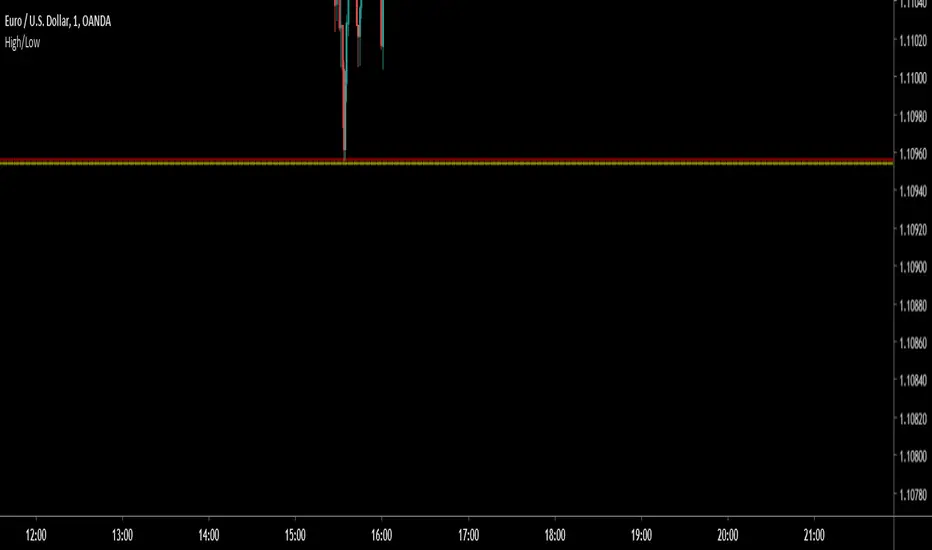
Fan Projections [theEccentricTrader]█ OVERVIEW
This indicator automatically projects trendlines in the shape of a fan, from a single point of origin. In the example above I have applied the indicator twice to the 1D SPXUSD. The seven upper lines (green) are projected at an angle of -5 from the 1-month swing high anchor point. And the five lower lines (blue) are projected at an angle of 10 from the 1-week swing low anchor point.
█ CONCEPTS
Green and Red Candles
• A green candle is one that closes with a high price equal to or above the price it opened.
• A red candle is one that closes with a low price that is lower than the price it opened.
Swing Highs and Swing Lows
• A swing high is a green candle or series of consecutive green candles followed by a single red candle to complete the swing and form the peak.
• A swing low is a red candle or series of consecutive red candles followed by a single green candle to complete the swing and form the trough.
Peak and Trough Prices (Basic)
• The peak price of a complete swing high is the high price of either the red candle that completes the swing high or the high price of the preceding green candle, depending on which is higher.
• The trough price of a complete swing low is the low price of either the green candle that completes the swing low or the low price of the preceding red candle, depending on which is lower.
Historic Peaks and Troughs
The current, or most recent, peak and trough occurrences are referred to as occurrence zero. Previous peak and trough occurrences are referred to as historic and ordered numerically from right to left, with the most recent historic peak and trough occurrences being occurrence one.
Support and Resistance
• Support refers to a price level where the demand for an asset is strong enough to prevent the price from falling further.
• Resistance refers to a price level where the supply of an asset is strong enough to prevent the price from rising further.
Support and resistance levels are important because they can help traders identify where the price of an asset might pause or reverse its direction, offering potential entry and exit points. For example, a trader might look to buy an asset when it approaches a support level , with the expectation that the price will bounce back up. Alternatively, a trader might look to sell an asset when it approaches a resistance level , with the expectation that the price will drop back down.
It's important to note that support and resistance levels are not always relevant, and the price of an asset can also break through these levels and continue moving in the same direction.
Trendlines
Trendlines are straight lines that are drawn between two or more points on a price chart. These lines are used as dynamic support and resistance levels for making strategic decisions and predictions about future price movements. For example traders will look for price movements along, and reactions to, trendlines in the form of rejections or breakouts/downs.
█ FEATURES
Inputs
• Anchor Point Type
• Swing High/Low Occurrence
• HTF Resolution
• Highest High/Lowest Low Lookback
• Angle Degree
• Number Lines
• Line Color
Anchor Point Types
• Swing High
• Swing Low
• Swing High (HTF)
• Swing Low (HTF)
• Highest High
• Lowest Low
• Intraday Highest High (intraday charts only)
• Intraday Lowest Low (intraday charts only)
Swing High/Swing Low Occurrence
This input is used to determine which historic peak or trough to reference for swing high or swing low anchor point types.
HTF Resolution
This input is used to determine which higher timeframe to reference for swing high (HTF) or swing low (HTF) anchor point types.
Highest High/Lowest Low Lookback
This input is used to determine the lookback length for highest high or lowest low anchor point types.
Intraday Highest High/Lowest Low Lookback
When using intraday highest high or lowest low anchor point types, the lookback length is calculated automatically based on number of bars since the daily candle opened.
Angle Degree
This input is used to determine the angle of the trendlines. The output is expressed in terms of point or pips, depending on the symbol type, which is then passed through the built in math.todegrees() function. Positive numbers will project the lines upwards while negative numbers will project the lines downwards. Depending on the market and timeframe, the impact input values will have on the visible gaps between the lines will vary greatly. For example, an input of 10 will have a far greater impact on the gaps between the lines when viewed from the 1-minute timeframe than it would on the 1-day timeframe. The input is a float and as such the value passed through can go into as many decimal places as the user requires.
It is also worth mentioning that as more lines are added the gaps between the lines, that are closest to the anchor point, will get tighter as they make their way up the y-axis. Although the gaps between the lines will stay constant at the x2 plot, i.e. a distance of 10 points between them, they will gradually get tighter and tighter at the point of origin as the slope of the lines get steeper.
Number Lines
This input is used to determine the number of lines to be drawn on the chart, maximum is 500.
█ LIMITATIONS
All green and red candle calculations are based on differences between open and close prices, as such I have made no attempt to account for green candles that gap lower and close below the close price of the preceding candle, or red candles that gap higher and close above the close price of the preceding candle. This may cause some unexpected behaviour on some markets and timeframes. I can only recommend using 24-hour markets, if and where possible, as there are far fewer gaps and, generally, more data to work with.
If the lines do not draw or you see a study error saying that the script references too many candles in history, this is most likely because the higher timeframe anchor point is not present on the current timeframe. This problem usually occurs when referencing a higher timeframe, such as the 1-month, from a much lower timeframe, such as the 1-minute. How far you can lookback for higher timeframe anchor points on the current timeframe will also be limited by your Trading View subscription plan. Premium users get 20,000 candles worth of data, pro+ and pro users get 10,000, and basic users get 5,000.
█ RAMBLINGS
It is my current thesis that the indicator will work best when used in conjunction with my Wavemeter indicator, which can be used to set the angle. For example, the average wave height or amplitude could be used as the value for the angle input. Or some factor or multiple of such an average. I think this makes sense as it allows for objectivity when applying the indicator across different markets and timeframes with different energies and vibrations.
“If you want to find the secrets of the universe, think in terms of energy, frequency and vibration.”
― Nikola Tesla
스크립트에서 "high low"에 대해 찾기
Swing Counter [theEccentricTrader]█ OVERVIEW
This indicator counts the number of confirmed swing high and swing low scenarios on any given candlestick chart and displays the statistics in a table, which can be repositioned and resized at the user's discretion.
█ CONCEPTS
Green and Red Candles
• A green candle is one that closes with a high price equal to or above the price it opened.
• A red candle is one that closes with a low price that is lower than the price it opened.
Swing Highs and Swing Lows
• A swing high is a green candle or series of consecutive green candles followed by a single red candle to complete the swing and form the peak.
• A swing low is a red candle or series of consecutive red candles followed by a single green candle to complete the swing and form the trough.
Peak and Trough Prices (Basic)
• The peak price of a complete swing high is the high price of either the red candle that completes the swing high or the high price of the preceding green candle, depending on which is higher.
• The trough price of a complete swing low is the low price of either the green candle that completes the swing low or the low price of the preceding red candle, depending on which is lower.
Peak and Trough Prices (Advanced)
• The advanced peak price of a complete swing high is the high price of either the red candle that completes the swing high or the high price of the highest preceding green candle high price, depending on which is higher.
• The advanced trough price of a complete swing low is the low price of either the green candle that completes the swing low or the low price of the lowest preceding red candle low price, depending on which is lower.
Green and Red Peaks and Troughs
• A green peak is one that derives its price from the green candle/s that constitute the swing high.
• A red peak is one that derives its price from the red candle that completes the swing high.
• A green trough is one that derives its price from the green candle that completes the swing low.
• A red trough is one that derives its price from the red candle/s that constitute the swing low.
Historic Peaks and Troughs
The current, or most recent, peak and trough occurrences are referred to as occurrence zero. Previous peak and trough occurrences are referred to as historic and ordered numerically from right to left, with the most recent historic peak and trough occurrences being occurrence one.
Upper Trends
• A return line uptrend is formed when the current peak price is higher than the preceding peak price.
• A downtrend is formed when the current peak price is lower than the preceding peak price.
• A double-top is formed when the current peak price is equal to the preceding peak price.
Lower Trends
• An uptrend is formed when the current trough price is higher than the preceding trough price.
• A return line downtrend is formed when the current trough price is lower than the preceding trough price.
• A double-bottom is formed when the current trough price is equal to the preceding trough price.
█ FEATURES
Inputs
• Start Date
• End Date
• Position
• Text Size
• Show Sample Period
• Show Plots
• Show Lines
Table
The table is colour coded, consists of three columns and nine rows. Blue cells denote neutral scenarios, green cells denote return line uptrend and uptrend scenarios, and red cells denote downtrend and return line downtrend scenarios.
The swing scenarios are listed in the first column with their corresponding total counts to the right, in the second column. The last row in column one, row nine, displays the sample period which can be adjusted or hidden via indicator settings.
Rows three and four in the third column of the table display the total higher peaks and higher troughs as percentages of total peaks and troughs, respectively. Rows five and six in the third column display the total lower peaks and lower troughs as percentages of total peaks and troughs, respectively. And rows seven and eight display the total double-top peaks and double-bottom troughs as percentages of total peaks and troughs, respectively.
Plots
I have added plots as a visual aid to the swing scenarios listed in the table. Green up-arrows with ‘HP’ denote higher peaks, while green up-arrows with ‘HT’ denote higher troughs. Red down-arrows with ‘LP’ denote higher peaks, while red down-arrows with ‘LT’ denote lower troughs. Similarly, blue diamonds with ‘DT’ denote double-top peaks and blue diamonds with ‘DB’ denote double-bottom troughs. These plots can be hidden via indicator settings.
Lines
I have also added green and red trendlines as a further visual aid to the swing scenarios listed in the table. Green lines denote return line uptrends (higher peaks) and uptrends (higher troughs), while red lines denote downtrends (lower peaks) and return line downtrends (lower troughs). These lines can be hidden via indicator settings.
█ HOW TO USE
This indicator is intended for research purposes and strategy development. I hope it will be useful in helping to gain a better understanding of the underlying dynamics at play on any given market and timeframe. It can, for example, give you an idea of any inherent biases such as a greater proportion of higher peaks to lower peaks. Or a greater proportion of higher troughs to lower troughs. Such information can be very useful when conducting top down analysis across multiple timeframes, or considering entry and exit methods.
What I find most fascinating about this logic, is that the number of swing highs and swing lows will always find equilibrium on each new complete wave cycle. If for example the chart begins with a swing high and ends with a swing low there will be an equal number of swing highs to swing lows. If the chart starts with a swing high and ends with a swing high there will be a difference of one between the two total values until another swing low is formed to complete the wave cycle sequence that began at start of the chart. Almost as if it was a fundamental truth of price action, although quite common sensical in many respects. As they say, what goes up must come down.
The objective logic for swing highs and swing lows I hope will form somewhat of a foundational building block for traders, researchers and developers alike. Not only does it facilitate the objective study of swing highs and swing lows it also facilitates that of ranges, trends, double trends, multi-part trends and patterns. The logic can also be used for objective anchor points. Concepts I will introduce and develop further in future publications.
█ LIMITATIONS
Some higher timeframe candles on tickers with larger lookbacks such as the DXY , do not actually contain all the open, high, low and close (OHLC) data at the beginning of the chart. Instead, they use the close price for open, high and low prices. So, while we can determine whether the close price is higher or lower than the preceding close price, there is no way of knowing what actually happened intra-bar for these candles. And by default candles that close at the same price as the open price, will be counted as green. You can avoid this problem by utilising the sample period filter.
The green and red candle calculations are based solely on differences between open and close prices, as such I have made no attempt to account for green candles that gap lower and close below the close price of the preceding candle, or red candles that gap higher and close above the close price of the preceding candle. I can only recommend using 24-hour markets, if and where possible, as there are far fewer gaps and, generally, more data to work with. Alternatively, you can replace the scenarios with your own logic to account for the gap anomalies, if you are feeling up to the challenge.
The sample size will be limited to your Trading View subscription plan. Premium users get 20,000 candles worth of data, pro+ and pro users get 10,000, and basic users get 5,000. If upgrading is currently not an option, you can always keep a rolling tally of the statistics in an excel spreadsheet or something of the like.
█ NOTES
I feel it important to address the mention of advanced peak and trough price logic. While I have introduced the concept, I have not included the logic in my script for a number of reasons. The most pertinent of which being the amount of extra work I would have to do to include it in a public release versus the actual difference it would make to the statistics. Based on my experience, there are actually only a small number of cases where the advanced peak and trough prices are different from the basic peak and trough prices. And with adequate multi-timeframe analysis any high or low prices that are not captured using basic peak and trough price logic on any given time frame, will no doubt be captured on a higher timeframe. See the example below on the 1H FOREXCOM:USDJPY chart (Figure 1), where the basic peak price logic denoted by the indicator plot does not capture what would be the advanced peak price, but on the 2H FOREXCOM:USDJPY chart (Figure 2), the basic peak logic does capture the advanced peak price from the 1H timeframe.
Figure 1.
Figure 2.
█ RAMBLINGS
“Never was there an age that placed economic interests higher than does our own. Never was the need of a scientific foundation for economic affairs felt more generally or more acutely. And never was the ability of practical men to utilize the achievements of science, in all fields of human activity, greater than in our day. If practical men, therefore, rely wholly on their own experience, and disregard our science in its present state of development, it cannot be due to a lack of serious interest or ability on their part. Nor can their disregard be the result of a haughty rejection of the deeper insight a true science would give into the circumstances and relationships determining the outcome of their activity. The cause of such remarkable indifference must not be sought elsewhere than in the present state of our science itself, in the sterility of all past endeavours to find its empirical foundations.” (Menger, 1871, p.45).
█ BIBLIOGRAPHY
Menger, C. (1871) Principles of Economics. Reprint, Auburn, Alabama: Ludwig Von Mises Institute: 2007.
Larry Williams Strategies IndicatorThis indicator is a trend following indicator. It plots some of the trend following strategies described by Larry Williams in his book 'Long Term Secrets to Short Term Trading'. Below are types of trend following strategies you can trade using this indicator. These are notes taken directly from Larry Williams' book.
Short Term Low Strategy
Short Term Low - Any daily low with higher lows on each side of it.
Intermediate Term Low – Any short term low with higher short term lows on each side of it.
Long Term Low – Any intermediate term low with higher intermediate term lows on each side of it.
Conceptual pattern for best buying opportunity is when forming an intermediate term low higher than the last intermediate term low.
This setup can be used on all time frames. However since Larry Williams usually trades the daily chart, the daily chart is probably the best timeframe to trade using this strategy.
Entry point – High of the day that has a higher high on the right side of it.
(My interpretation: price crossing above the high of the previous day is the buy signal)
Target – Markets have a strong tendency to rally above the last intermediate term high by the same amount it moved from the last intermediate term high to the lowest point prior to advancing to new highs.
Trailing Stop – Set stop to most recent short term low, move up as new short term lows are formed. Can also use formation of next intermediate term high as an exit point.
A 'run' to the upside is over when price fails to move higher the next day and falls below the prior day's low.
Short Term High Strategy
Short Term High - Any daily high with lower highs on each side of it.
Intermediate Term High – Any short term high with lower short term highs on each side of it.
Long Term High – Any intermediate term high with lower intermediate term highs on each side of it.
Conceptual pattern for best selling opportunity is when forming an intermediate term high lower than the last intermediate term high.
This setup can be used on all time frames. However since Larry Williams usually trades the daily chart, the daily chart is probably the best timeframe to trade using this strategy.
Entry point – Low of the day that has a lower low on the right side of it.
(My interpretation: price crossing below the low of the previous day is the sell short signal)
Target – Markets have a strong tendency to fall below the last intermediate term low by the same amount it moved from the last intermediate term low to the highest point prior to declining to new lows.
Trailing Stop – Set stop to most recent short term high, move down as new short term highs are formed. Can also use formation of next intermediate term low as an exit point.
A 'run' to the downside is over when price fails to move lower the next day and rises above the prior day's high.
Trend Reversals
A trend change from down to up occurs when a short term high is exceeded on the upside, a trend change from up to down is identified by price going below the most recent low.
Can take these signals to make trades, but it is best to filter them with a confirmation or edge such as Trading Day of the Week, Trading Day of the Month, trendlines, etc. to cut down on false signals.
Three Bar High/Low System
Calculate a three bar moving average of the highs and a three bar moving average of the lows.
Strategy is to buy at the at the price of the three bar moving average of the lows - if the trend is positive according to the swing point trend identification technique - and take profits at the three bar moving average of the highs.
Selling is just the opposite. Sell short at the three bar moving average of the highs and take profits at the three bar moving average of the lows, using the trend identification technique above for confirmation.
This strategy can work on any timeframe, but was described as a daytrading system by Larry Williams.
Contrarian Period High & LowContrarian Period High & Low
This indicator pairs nicely with the Contrarian 100 MA and can be located here:
Overview
The "Contrarian Period High & Low" indicator is a powerful technical analysis tool designed for traders seeking to identify key support and resistance levels and capitalize on contrarian trading opportunities. By tracking the highest highs and lowest lows over user-defined periods (Daily, Weekly, or Monthly), this indicator plots historical levels and generates buy and sell signals when price breaks these levels in a contrarian manner. A unique blue dot counter and action table enhance decision-making, making it ideal for swing traders, trend followers, and those trading forex, stocks, or cryptocurrencies. Optimized for daily charts, it can be adapted to other timeframes with proper testing.
How It Works
The indicator identifies the highest high and lowest low within a specified period (e.g., daily, weekly, or monthly) and draws horizontal lines for the previous period’s extremes on the chart. These levels act as dynamic support and resistance zones. Contrarian signals are generated when the price crosses below the previous period’s low (buy signal) or above the previous period’s high (sell signal), indicating potential reversals. A blue dot counter tracks consecutive buy signals, and a table displays the count and recommended action, helping traders decide whether to hold or flip positions.
Key Components
Period High/Low Levels: Tracks the highest high and lowest low for each period, plotting red lines for highs and green lines for lows from the bar where they occurred, extending for a user-defined length (default: 200 bars).
Contrarian Signals: Generates buy signals (blue circles) when price crosses below the previous period’s low and sell signals (white circles) when price crosses above the previous period’s high, designed to capture potential reversals.
Blue Dot Tracker: Counts consecutive buy signals (“blue dots”). If three or more occur, it suggests a stronger trend, with the table recommending whether to “Hold Investment” or “Flip Investment.”
Action Table: A 2x2 table in the bottom-right corner displays the blue dot count and action (“Hold Investment” if count ≥ 4, else “Flip Investment”) for quick reference.
Mathematical Concepts
Period Detection: Uses an approximate bar count to define periods (1 bar for Daily, 5 bars for Weekly, 20 bars for Monthly on a daily chart). When a new period starts, the previous period’s high/low is finalized and plotted.
High/Low Tracking:
Highest high (periodHigh) and lowest low (periodLow) are updated within the period.
Lines are drawn at these levels when the period ends, starting from the bar where the extreme occurred (periodHighBar, periodLowBar).
Signal Logic:
Buy signal: ta.crossunder(close , prevPeriodLow) and not lowBroken and barstate.isconfirmed
Sell signal: ta.crossover(close , prevPeriodHigh) and not highBroken and barstate.isconfirmed
Flags (highBroken, lowBroken) prevent multiple signals for the same level within a period.
Blue Dot Counter: Increments on each buy signal, resets on a sell signal or if price exceeds the entry price after three or more buy signals.
Entry and Exit Rules
Buy Signal (Blue Circle): Triggered when the price crosses below the previous period’s low, suggesting a potential oversold condition and buying opportunity. The signal appears as a blue circle below the price bar.
Sell Signal (White Circle): Triggered when the price crosses above the previous period’s high, indicating a potential overbought condition and selling opportunity. The signal appears as a white circle above the price bar.
Blue Dot Tracker:
Increments blueDotCount on each buy signal and sets an entryPrice on the first buy.
Resets on a sell signal or if price exceeds entryPrice after three or more buy signals.
If blueDotCount >= 3, the table suggests holding; if >= 4, it reinforces “Hold Investment.”
Exit Rules: Exit a buy position on a sell signal or when price exceeds the entry price after three or more buy signals. Combine with other tools (e.g., trendlines, support/resistance) for additional confirmation. Always apply proper risk management.
Recommended Usage
The "Contrarian Period High & Low" indicator is optimized for daily charts but can be adapted to other timeframes (e.g., 1H, 4H) with adjustments to the period bar count. It excels in markets with clear support/resistance levels and potential reversal zones. Traders should:
Backtest the indicator on their chosen asset and timeframe to validate signal reliability.
Combine with other technical tools (e.g., moving averages, Fibonacci levels) for stronger trade confirmation.
Adjust barsPerPeriod (e.g., ~120 bars for Weekly on hourly charts) based on the chart timeframe and market volatility.
Monitor the action table to guide position management based on blue dot counts.
Customization Options
Period Type: Choose between Daily, Weekly, or Monthly periods (default: Monthly).
Line Length: Set the length of high/low lines in bars (default: 200).
Show Highs/Lows: Toggle visibility of period high (red) and low (green) lines.
Max Lines to Keep: Limit the number of historical lines displayed (default: 10).
Hide Signals: Toggle buy/sell signal visibility for a cleaner chart.
Table Display: A fixed table in the bottom-right corner shows the blue dot count and action, with yellow (Hold) or green (Flip) backgrounds based on the count.
Why Use This Indicator?
The "Contrarian Period High & Low" indicator offers a unique blend of support/resistance visualization and contrarian signal generation, making it a versatile tool for identifying potential reversals. Its clear visual cues (lines and signals), blue dot tracker, and actionable table provide traders with an intuitive way to monitor market structure and manage trades. Whether you’re a beginner or an experienced trader, this indicator enhances your ability to spot key levels and time entries/exits effectively.
Tips for Users
Test the indicator thoroughly on your chosen market and timeframe to optimize settings (e.g., adjust barsPerPeriod for non-daily charts).
Use in conjunction with price action or other indicators for stronger trade setups.
Monitor the action table to decide whether to hold or flip positions based on blue dot counts.
Ensure your chart timeframe aligns with the selected period type (e.g., daily chart for Monthly periods).
Apply strict risk management to protect against false breakouts.
Happy trading with the Contrarian Period High & Low indicator! Share your feedback and strategies in the TradingView community!
PriceActionLibrary "PriceAction"
Hi all!
This library will help you to plot the market structure and liquidity. By now, the only part in the price action section is liquidity, but I plan to add more later on. The market structure will be split into two parts, 'Internal' and 'Swing' with separate pivot lengths. For these two trends it will show you:
• Break of structure (BOS)
• Change of character (CHoCH/CHoCH+) (mandatory)
• Equal high/low (EQH/EQL)
It's inspired by "Smart Money Concepts (SMC) " by LuxAlgo.
This library is now the same code as the code in my library 'MarketStructure', but it has evolved into a more price action oriented library than just a market structure library. This is more accurate and I will continue working on this library to keep it growing.
This code does not provide any examples, but you can look at my indicators 'Market structure' () and 'Order blocks' (), where I use the 'MarketStructure' library (which is the same code).
Market structure
Both of these market structures can be enabled/disabled by setting them to 'na'. The pivots lengths can be configured separately. The pivots found will be the 'base' of and will show you when price breaks it. When that happens a break of structure or a change of character will be created. The latest 5 pivots found within the current trends will be kept to take action on. They are cleared on a change of character, so nothing (break of structures or change of characters) can happen on pivots before a trend change. The internal market structure is shown with dashed lines and swing market structure is shown with solid lines.
Labels for a change of character can have either the text 'CHoCH' or 'CHoCH+'. A Change of Character plus is formed when price fails to form a higher high or a lower low before reversing. Note that a pivot that is created after the change of character might have a higher high or a lower low, thus not making the break a 'CHoCH+'. This is not changed after the pivot is found but is kept as is.
A break of structure is removed if an earlier pivot within the same trend is broken, i.e. another break of structure (with a longer distance) is created. Like in the images below, the first pivot (in the first image) is removed when an earlier pivot's higher price within the same trend is broken (the second image):
[image [https://www.tradingview.com/x/PRP6YtPA/
Equal high/lows have a configurable color setting and can be configured to be extended to the right. Equal high/lows are only possible if it's not been broken by price. A factor (percentage of width) of the Average True Length (of length 14) that the pivot must be within to to be considered an Equal high/low. Equal highs/lows can be of 2 pivots or more.
You are able to show the pivots that are used. "HH" (higher high), "HL" (higher low), "LH" (lower high), "LL" (lower low) and "H"/"L" (for pivots (high/low) when the trend has changed) are the labels used. There are also labels for break of structures ('BOS') and change of characters ('CHoCH' or 'CHoCH+'). The size of these texts is set in the 'FontSize' setting.
When programming I focused on simplicity and ease of read. I did not focus on performance, I will do so if it's a problem (haven't noticed it is one yet).
You can set alerts for when a change of character, break of structure or an equal high/low (new or an addition to a previously found) happens. The alerts that are fired are on 'once_per_bar_close' to avoid repainting. This has the drawback to alert you when the bar closes.
Price action
The indicator will create lines and zones for spotted liquidity. It will draw a line (with dotted style) at the price level that was liquidated, but it will also draw a zone from that level to the bar that broke the pivot high or low price. If that zone is large the liquidation is big and might be significant. This can be disabled in the settings. You can also change the confirmation candles (that does not close above or below the pivot level) needed after a liquidation and how many pivots back to look at.
The lines and boxes drawn will look like this if the color is orange:
Hope this is of help!
Will draw out the market structure for the disired pivot length.
Liqudity(liquidity)
Will draw liquidity.
Parameters:
liquidity (Liquidity) : The 'PriceAction.Liquidity' object.
Pivot(structure)
Sets the pivots in the structure.
Parameters:
structure (Structure)
PivotLabels(structure)
Draws labels for the pivots found.
Parameters:
structure (Structure)
EqualHighOrLow(structure)
Draws the boxes for equal highs/lows. Also creates labels for the pivots included.
Parameters:
structure (Structure)
BreakOfStructure(structure)
Will create lines when a break of strycture occures.
Parameters:
structure (Structure)
Returns: A boolean that represents if a break of structure was found or not.
ChangeOfCharacter(structure)
Will create lines when a change of character occures. This line will have a label with "CHoCH" or "CHoCH+".
Parameters:
structure (Structure)
Returns: A boolean that represents if a change of character was found or not.
VisualizeCurrent(structure)
Will create a box with a background for between the latest high and low pivots. This can be used as the current trading range (if the pivots broke strucure somehow).
Parameters:
structure (Structure)
StructureBreak
Holds drawings for a structure break.
Fields:
Line (series line) : The line object.
Label (series label) : The label object.
Pivot
Holds all the values for a found pivot.
Fields:
Price (series float) : The price of the pivot.
BarIndex (series int) : The bar_index where the pivot occured.
Type (series int) : The type of the pivot (-1 = low, 1 = high).
Time (series int) : The time where the pivot occured.
BreakOfStructureBroken (series bool) : Sets to true if a break of structure has happened.
LiquidityBroken (series bool) : Sets to true if a liquidity of the price level has happened.
ChangeOfCharacterBroken (series bool) : Sets to true if a change of character has happened.
Structure
Holds all the values for the market structure.
Fields:
LeftLength (series int) : Define the left length of the pivots used.
RightLength (series int) : Define the right length of the pivots used.
Type (series Type) : Set the type of the market structure. Two types can be used, 'internal' and 'swing' (0 = internal, 1 = swing).
Trend (series int) : This will be set internally and can be -1 = downtrend, 1 = uptrend.
EqualPivotsFactor (series float) : Set how the limits are for an equal pivot. This is a factor of the Average True Length (ATR) of length 14. If a low pivot is considered to be equal if it doesn't break the low pivot (is at a lower value) and is inside the previous low pivot + this limit.
ExtendEqualPivotsZones (series bool) : Set to true if you want the equal pivots zones to be extended.
ExtendEqualPivotsStyle (series string) : Set the style of equal pivot zones.
ExtendEqualPivotsColor (series color) : Set the color of equal pivot zones.
EqualHighs (array) : Holds the boxes for zones that contains equal highs.
EqualLows (array) : Holds the boxes for zones that contains equal lows.
BreakOfStructures (array) : Holds all the break of structures within the trend (before a change of character).
Pivots (array) : All the pivots in the current trend, added with the latest first, this is cleared when the trend changes.
FontSize (series int) : Holds the size of the font displayed.
AlertChangeOfCharacter (series bool) : Holds true or false if a change of character should be alerted or not.
AlertBreakOfStructure (series bool) : Holds true or false if a break of structure should be alerted or not.
AlerEqualPivots (series bool) : Holds true or false if equal highs/lows should be alerted or not.
Liquidity
Holds all the values for liquidity.
Fields:
LiquidityPivotsHigh (array) : All high pivots for liquidity.
LiquidityPivotsLow (array) : All low pivots for liquidity.
LiquidityConfirmationBars (series int) : The number of bars to confirm that a liquidity is valid.
LiquidityPivotsLookback (series int) : A number of pivots to look back for.
FontSize (series int) : Holds the size of the font displayed.
PriceAction
Holds all the values for the general price action and the market structures.
Fields:
Liquidity (Liquidity)
Swing (Structure) : Placeholder for all objects used for the swing market structure.
Internal (Structure) : Placeholder for all objects used for the internal market structure.
Markov Chain [3D] | FractalystWhat exactly is a Markov Chain?
This indicator uses a Markov Chain model to analyze, quantify, and visualize the transitions between market regimes (Bull, Bear, Neutral) on your chart. It dynamically detects these regimes in real-time, calculates transition probabilities, and displays them as animated 3D spheres and arrows, giving traders intuitive insight into current and future market conditions.
How does a Markov Chain work, and how should I read this spheres-and-arrows diagram?
Think of three weather modes: Sunny, Rainy, Cloudy.
Each sphere is one mode. The loop on a sphere means “stay the same next step” (e.g., Sunny again tomorrow).
The arrows leaving a sphere show where things usually go next if they change (e.g., Sunny moving to Cloudy).
Some paths matter more than others. A more prominent loop means the current mode tends to persist. A more prominent outgoing arrow means a change to that destination is the usual next step.
Direction isn’t symmetric: moving Sunny→Cloudy can behave differently than Cloudy→Sunny.
Now relabel the spheres to markets: Bull, Bear, Neutral.
Spheres: market regimes (uptrend, downtrend, range).
Self‑loop: tendency for the current regime to continue on the next bar.
Arrows: the most common next regime if a switch happens.
How to read: Start at the sphere that matches current bar state. If the loop stands out, expect continuation. If one outgoing path stands out, that switch is the typical next step. Opposite directions can differ (Bear→Neutral doesn’t have to match Neutral→Bear).
What states and transitions are shown?
The three market states visualized are:
Bullish (Bull): Upward or strong-market regime.
Bearish (Bear): Downward or weak-market regime.
Neutral: Sideways or range-bound regime.
Bidirectional animated arrows and probability labels show how likely the market is to move from one regime to another (e.g., Bull → Bear or Neutral → Bull).
How does the regime detection system work?
You can use either built-in price returns (based on adaptive Z-score normalization) or supply three custom indicators (such as volume, oscillators, etc.).
Values are statistically normalized (Z-scored) over a configurable lookback period.
The normalized outputs are classified into Bull, Bear, or Neutral zones.
If using three indicators, their regime signals are averaged and smoothed for robustness.
How are transition probabilities calculated?
On every confirmed bar, the algorithm tracks the sequence of detected market states, then builds a rolling window of transitions.
The code maintains a transition count matrix for all regime pairs (e.g., Bull → Bear).
Transition probabilities are extracted for each possible state change using Laplace smoothing for numerical stability, and frequently updated in real-time.
What is unique about the visualization?
3D animated spheres represent each regime and change visually when active.
Animated, bidirectional arrows reveal transition probabilities and allow you to see both dominant and less likely regime flows.
Particles (moving dots) animate along the arrows, enhancing the perception of regime flow direction and speed.
All elements dynamically update with each new price bar, providing a live market map in an intuitive, engaging format.
Can I use custom indicators for regime classification?
Yes! Enable the "Custom Indicators" switch and select any three chart series as inputs. These will be normalized and combined (each with equal weight), broadening the regime classification beyond just price-based movement.
What does the “Lookback Period” control?
Lookback Period (default: 100) sets how much historical data builds the probability matrix. Shorter periods adapt faster to regime changes but may be noisier. Longer periods are more stable but slower to adapt.
How is this different from a Hidden Markov Model (HMM)?
It sets the window for both regime detection and probability calculations. Lower values make the system more reactive, but potentially noisier. Higher values smooth estimates and make the system more robust.
How is this Markov Chain different from a Hidden Markov Model (HMM)?
Markov Chain (as here): All market regimes (Bull, Bear, Neutral) are directly observable on the chart. The transition matrix is built from actual detected regimes, keeping the model simple and interpretable.
Hidden Markov Model: The actual regimes are unobservable ("hidden") and must be inferred from market output or indicator "emissions" using statistical learning algorithms. HMMs are more complex, can capture more subtle structure, but are harder to visualize and require additional machine learning steps for training.
A standard Markov Chain models transitions between observable states using a simple transition matrix, while a Hidden Markov Model assumes the true states are hidden (latent) and must be inferred from observable “emissions” like price or volume data. In practical terms, a Markov Chain is transparent and easier to implement and interpret; an HMM is more expressive but requires statistical inference to estimate hidden states from data.
Markov Chain: states are observable; you directly count or estimate transition probabilities between visible states. This makes it simpler, faster, and easier to validate and tune.
HMM: states are hidden; you only observe emissions generated by those latent states. Learning involves machine learning/statistical algorithms (commonly Baum–Welch/EM for training and Viterbi for decoding) to infer both the transition dynamics and the most likely hidden state sequence from data.
How does the indicator avoid “repainting” or look-ahead bias?
All regime changes and matrix updates happen only on confirmed (closed) bars, so no future data is leaked, ensuring reliable real-time operation.
Are there practical tuning tips?
Tune the Lookback Period for your asset/timeframe: shorter for fast markets, longer for stability.
Use custom indicators if your asset has unique regime drivers.
Watch for rapid changes in transition probabilities as early warning of a possible regime shift.
Who is this indicator for?
Quants and quantitative researchers exploring probabilistic market modeling, especially those interested in regime-switching dynamics and Markov models.
Programmers and system developers who need a probabilistic regime filter for systematic and algorithmic backtesting:
The Markov Chain indicator is ideally suited for programmatic integration via its bias output (1 = Bull, 0 = Neutral, -1 = Bear).
Although the visualization is engaging, the core output is designed for automated, rules-based workflows—not for discretionary/manual trading decisions.
Developers can connect the indicator’s output directly to their Pine Script logic (using input.source()), allowing rapid and robust backtesting of regime-based strategies.
It acts as a plug-and-play regime filter: simply plug the bias output into your entry/exit logic, and you have a scientifically robust, probabilistically-derived signal for filtering, timing, position sizing, or risk regimes.
The MC's output is intentionally "trinary" (1/0/-1), focusing on clear regime states for unambiguous decision-making in code. If you require nuanced, multi-probability or soft-label state vectors, consider expanding the indicator or stacking it with a probability-weighted logic layer in your scripting.
Because it avoids subjectivity, this approach is optimal for systematic quants, algo developers building backtested, repeatable strategies based on probabilistic regime analysis.
What's the mathematical foundation behind this?
The mathematical foundation behind this Markov Chain indicator—and probabilistic regime detection in finance—draws from two principal models: the (standard) Markov Chain and the Hidden Markov Model (HMM).
How to use this indicator programmatically?
The Markov Chain indicator automatically exports a bias value (+1 for Bullish, -1 for Bearish, 0 for Neutral) as a plot visible in the Data Window. This allows you to integrate its regime signal into your own scripts and strategies for backtesting, automation, or live trading.
Step-by-Step Integration with Pine Script (input.source)
Add the Markov Chain indicator to your chart.
This must be done first, since your custom script will "pull" the bias signal from the indicator's plot.
In your strategy, create an input using input.source()
Example:
//@version=5
strategy("MC Bias Strategy Example")
mcBias = input.source(close, "MC Bias Source")
After saving, go to your script’s settings. For the “MC Bias Source” input, select the plot/output of the Markov Chain indicator (typically its bias plot).
Use the bias in your trading logic
Example (long only on Bull, flat otherwise):
if mcBias == 1
strategy.entry("Long", strategy.long)
else
strategy.close("Long")
For more advanced workflows, combine mcBias with additional filters or trailing stops.
How does this work behind-the-scenes?
TradingView’s input.source() lets you use any plot from another indicator as a real-time, “live” data feed in your own script (source).
The selected bias signal is available to your Pine code as a variable, enabling logical decisions based on regime (trend-following, mean-reversion, etc.).
This enables powerful strategy modularity : decouple regime detection from entry/exit logic, allowing fast experimentation without rewriting core signal code.
Integrating 45+ Indicators with Your Markov Chain — How & Why
The Enhanced Custom Indicators Export script exports a massive suite of over 45 technical indicators—ranging from classic momentum (RSI, MACD, Stochastic, etc.) to trend, volume, volatility, and oscillator tools—all pre-calculated, centered/scaled, and available as plots.
// Enhanced Custom Indicators Export - 45 Technical Indicators
// Comprehensive technical analysis suite for advanced market regime detection
//@version=6
indicator('Enhanced Custom Indicators Export | Fractalyst', shorttitle='Enhanced CI Export', overlay=false, scale=scale.right, max_labels_count=500, max_lines_count=500)
// |----- Input Parameters -----| //
momentum_group = "Momentum Indicators"
trend_group = "Trend Indicators"
volume_group = "Volume Indicators"
volatility_group = "Volatility Indicators"
oscillator_group = "Oscillator Indicators"
display_group = "Display Settings"
// Common lengths
length_14 = input.int(14, "Standard Length (14)", minval=1, maxval=100, group=momentum_group)
length_20 = input.int(20, "Medium Length (20)", minval=1, maxval=200, group=trend_group)
length_50 = input.int(50, "Long Length (50)", minval=1, maxval=200, group=trend_group)
// Display options
show_table = input.bool(true, "Show Values Table", group=display_group)
table_size = input.string("Small", "Table Size", options= , group=display_group)
// |----- MOMENTUM INDICATORS (15 indicators) -----| //
// 1. RSI (Relative Strength Index)
rsi_14 = ta.rsi(close, length_14)
rsi_centered = rsi_14 - 50
// 2. Stochastic Oscillator
stoch_k = ta.stoch(close, high, low, length_14)
stoch_d = ta.sma(stoch_k, 3)
stoch_centered = stoch_k - 50
// 3. Williams %R
williams_r = ta.stoch(close, high, low, length_14) - 100
// 4. MACD (Moving Average Convergence Divergence)
= ta.macd(close, 12, 26, 9)
// 5. Momentum (Rate of Change)
momentum = ta.mom(close, length_14)
momentum_pct = (momentum / close ) * 100
// 6. Rate of Change (ROC)
roc = ta.roc(close, length_14)
// 7. Commodity Channel Index (CCI)
cci = ta.cci(close, length_20)
// 8. Money Flow Index (MFI)
mfi = ta.mfi(close, length_14)
mfi_centered = mfi - 50
// 9. Awesome Oscillator (AO)
ao = ta.sma(hl2, 5) - ta.sma(hl2, 34)
// 10. Accelerator Oscillator (AC)
ac = ao - ta.sma(ao, 5)
// 11. Chande Momentum Oscillator (CMO)
cmo = ta.cmo(close, length_14)
// 12. Detrended Price Oscillator (DPO)
dpo = close - ta.sma(close, length_20)
// 13. Price Oscillator (PPO)
ppo = ta.sma(close, 12) - ta.sma(close, 26)
ppo_pct = (ppo / ta.sma(close, 26)) * 100
// 14. TRIX
trix_ema1 = ta.ema(close, length_14)
trix_ema2 = ta.ema(trix_ema1, length_14)
trix_ema3 = ta.ema(trix_ema2, length_14)
trix = ta.roc(trix_ema3, 1) * 10000
// 15. Klinger Oscillator
klinger = ta.ema(volume * (high + low + close) / 3, 34) - ta.ema(volume * (high + low + close) / 3, 55)
// 16. Fisher Transform
fisher_hl2 = 0.5 * (hl2 - ta.lowest(hl2, 10)) / (ta.highest(hl2, 10) - ta.lowest(hl2, 10)) - 0.25
fisher = 0.5 * math.log((1 + fisher_hl2) / (1 - fisher_hl2))
// 17. Stochastic RSI
stoch_rsi = ta.stoch(rsi_14, rsi_14, rsi_14, length_14)
stoch_rsi_centered = stoch_rsi - 50
// 18. Relative Vigor Index (RVI)
rvi_num = ta.swma(close - open)
rvi_den = ta.swma(high - low)
rvi = rvi_den != 0 ? rvi_num / rvi_den : 0
// 19. Balance of Power (BOP)
bop = (close - open) / (high - low)
// |----- TREND INDICATORS (10 indicators) -----| //
// 20. Simple Moving Average Momentum
sma_20 = ta.sma(close, length_20)
sma_momentum = ((close - sma_20) / sma_20) * 100
// 21. Exponential Moving Average Momentum
ema_20 = ta.ema(close, length_20)
ema_momentum = ((close - ema_20) / ema_20) * 100
// 22. Parabolic SAR
sar = ta.sar(0.02, 0.02, 0.2)
sar_trend = close > sar ? 1 : -1
// 23. Linear Regression Slope
lr_slope = ta.linreg(close, length_20, 0) - ta.linreg(close, length_20, 1)
// 24. Moving Average Convergence (MAC)
mac = ta.sma(close, 10) - ta.sma(close, 30)
// 25. Trend Intensity Index (TII)
tii_sum = 0.0
for i = 1 to length_20
tii_sum += close > close ? 1 : 0
tii = (tii_sum / length_20) * 100
// 26. Ichimoku Cloud Components
ichimoku_tenkan = (ta.highest(high, 9) + ta.lowest(low, 9)) / 2
ichimoku_kijun = (ta.highest(high, 26) + ta.lowest(low, 26)) / 2
ichimoku_signal = ichimoku_tenkan > ichimoku_kijun ? 1 : -1
// 27. MESA Adaptive Moving Average (MAMA)
mama_alpha = 2.0 / (length_20 + 1)
mama = ta.ema(close, length_20)
mama_momentum = ((close - mama) / mama) * 100
// 28. Zero Lag Exponential Moving Average (ZLEMA)
zlema_lag = math.round((length_20 - 1) / 2)
zlema_data = close + (close - close )
zlema = ta.ema(zlema_data, length_20)
zlema_momentum = ((close - zlema) / zlema) * 100
// |----- VOLUME INDICATORS (6 indicators) -----| //
// 29. On-Balance Volume (OBV)
obv = ta.obv
// 30. Volume Rate of Change (VROC)
vroc = ta.roc(volume, length_14)
// 31. Price Volume Trend (PVT)
pvt = ta.pvt
// 32. Negative Volume Index (NVI)
nvi = 0.0
nvi := volume < volume ? nvi + ((close - close ) / close ) * nvi : nvi
// 33. Positive Volume Index (PVI)
pvi = 0.0
pvi := volume > volume ? pvi + ((close - close ) / close ) * pvi : pvi
// 34. Volume Oscillator
vol_osc = ta.sma(volume, 5) - ta.sma(volume, 10)
// 35. Ease of Movement (EOM)
eom_distance = high - low
eom_box_height = volume / 1000000
eom = eom_box_height != 0 ? eom_distance / eom_box_height : 0
eom_sma = ta.sma(eom, length_14)
// 36. Force Index
force_index = volume * (close - close )
force_index_sma = ta.sma(force_index, length_14)
// |----- VOLATILITY INDICATORS (10 indicators) -----| //
// 37. Average True Range (ATR)
atr = ta.atr(length_14)
atr_pct = (atr / close) * 100
// 38. Bollinger Bands Position
bb_basis = ta.sma(close, length_20)
bb_dev = 2.0 * ta.stdev(close, length_20)
bb_upper = bb_basis + bb_dev
bb_lower = bb_basis - bb_dev
bb_position = bb_dev != 0 ? (close - bb_basis) / bb_dev : 0
bb_width = bb_dev != 0 ? (bb_upper - bb_lower) / bb_basis * 100 : 0
// 39. Keltner Channels Position
kc_basis = ta.ema(close, length_20)
kc_range = ta.ema(ta.tr, length_20)
kc_upper = kc_basis + (2.0 * kc_range)
kc_lower = kc_basis - (2.0 * kc_range)
kc_position = kc_range != 0 ? (close - kc_basis) / kc_range : 0
// 40. Donchian Channels Position
dc_upper = ta.highest(high, length_20)
dc_lower = ta.lowest(low, length_20)
dc_basis = (dc_upper + dc_lower) / 2
dc_position = (dc_upper - dc_lower) != 0 ? (close - dc_basis) / (dc_upper - dc_lower) : 0
// 41. Standard Deviation
std_dev = ta.stdev(close, length_20)
std_dev_pct = (std_dev / close) * 100
// 42. Relative Volatility Index (RVI)
rvi_up = ta.stdev(close > close ? close : 0, length_14)
rvi_down = ta.stdev(close < close ? close : 0, length_14)
rvi_total = rvi_up + rvi_down
rvi_volatility = rvi_total != 0 ? (rvi_up / rvi_total) * 100 : 50
// 43. Historical Volatility
hv_returns = math.log(close / close )
hv = ta.stdev(hv_returns, length_20) * math.sqrt(252) * 100
// 44. Garman-Klass Volatility
gk_vol = math.log(high/low) * math.log(high/low) - (2*math.log(2)-1) * math.log(close/open) * math.log(close/open)
gk_volatility = math.sqrt(ta.sma(gk_vol, length_20)) * 100
// 45. Parkinson Volatility
park_vol = math.log(high/low) * math.log(high/low)
parkinson = math.sqrt(ta.sma(park_vol, length_20) / (4 * math.log(2))) * 100
// 46. Rogers-Satchell Volatility
rs_vol = math.log(high/close) * math.log(high/open) + math.log(low/close) * math.log(low/open)
rogers_satchell = math.sqrt(ta.sma(rs_vol, length_20)) * 100
// |----- OSCILLATOR INDICATORS (5 indicators) -----| //
// 47. Elder Ray Index
elder_bull = high - ta.ema(close, 13)
elder_bear = low - ta.ema(close, 13)
elder_power = elder_bull + elder_bear
// 48. Schaff Trend Cycle (STC)
stc_macd = ta.ema(close, 23) - ta.ema(close, 50)
stc_k = ta.stoch(stc_macd, stc_macd, stc_macd, 10)
stc_d = ta.ema(stc_k, 3)
stc = ta.stoch(stc_d, stc_d, stc_d, 10)
// 49. Coppock Curve
coppock_roc1 = ta.roc(close, 14)
coppock_roc2 = ta.roc(close, 11)
coppock = ta.wma(coppock_roc1 + coppock_roc2, 10)
// 50. Know Sure Thing (KST)
kst_roc1 = ta.roc(close, 10)
kst_roc2 = ta.roc(close, 15)
kst_roc3 = ta.roc(close, 20)
kst_roc4 = ta.roc(close, 30)
kst = ta.sma(kst_roc1, 10) + 2*ta.sma(kst_roc2, 10) + 3*ta.sma(kst_roc3, 10) + 4*ta.sma(kst_roc4, 15)
// 51. Percentage Price Oscillator (PPO)
ppo_line = ((ta.ema(close, 12) - ta.ema(close, 26)) / ta.ema(close, 26)) * 100
ppo_signal = ta.ema(ppo_line, 9)
ppo_histogram = ppo_line - ppo_signal
// |----- PLOT MAIN INDICATORS -----| //
// Plot key momentum indicators
plot(rsi_centered, title="01_RSI_Centered", color=color.purple, linewidth=1)
plot(stoch_centered, title="02_Stoch_Centered", color=color.blue, linewidth=1)
plot(williams_r, title="03_Williams_R", color=color.red, linewidth=1)
plot(macd_histogram, title="04_MACD_Histogram", color=color.orange, linewidth=1)
plot(cci, title="05_CCI", color=color.green, linewidth=1)
// Plot trend indicators
plot(sma_momentum, title="06_SMA_Momentum", color=color.navy, linewidth=1)
plot(ema_momentum, title="07_EMA_Momentum", color=color.maroon, linewidth=1)
plot(sar_trend, title="08_SAR_Trend", color=color.teal, linewidth=1)
plot(lr_slope, title="09_LR_Slope", color=color.lime, linewidth=1)
plot(mac, title="10_MAC", color=color.fuchsia, linewidth=1)
// Plot volatility indicators
plot(atr_pct, title="11_ATR_Pct", color=color.yellow, linewidth=1)
plot(bb_position, title="12_BB_Position", color=color.aqua, linewidth=1)
plot(kc_position, title="13_KC_Position", color=color.olive, linewidth=1)
plot(std_dev_pct, title="14_StdDev_Pct", color=color.silver, linewidth=1)
plot(bb_width, title="15_BB_Width", color=color.gray, linewidth=1)
// Plot volume indicators
plot(vroc, title="16_VROC", color=color.blue, linewidth=1)
plot(eom_sma, title="17_EOM", color=color.red, linewidth=1)
plot(vol_osc, title="18_Vol_Osc", color=color.green, linewidth=1)
plot(force_index_sma, title="19_Force_Index", color=color.orange, linewidth=1)
plot(obv, title="20_OBV", color=color.purple, linewidth=1)
// Plot additional oscillators
plot(ao, title="21_Awesome_Osc", color=color.navy, linewidth=1)
plot(cmo, title="22_CMO", color=color.maroon, linewidth=1)
plot(dpo, title="23_DPO", color=color.teal, linewidth=1)
plot(trix, title="24_TRIX", color=color.lime, linewidth=1)
plot(fisher, title="25_Fisher", color=color.fuchsia, linewidth=1)
// Plot more momentum indicators
plot(mfi_centered, title="26_MFI_Centered", color=color.yellow, linewidth=1)
plot(ac, title="27_AC", color=color.aqua, linewidth=1)
plot(ppo_pct, title="28_PPO_Pct", color=color.olive, linewidth=1)
plot(stoch_rsi_centered, title="29_StochRSI_Centered", color=color.silver, linewidth=1)
plot(klinger, title="30_Klinger", color=color.gray, linewidth=1)
// Plot trend continuation
plot(tii, title="31_TII", color=color.blue, linewidth=1)
plot(ichimoku_signal, title="32_Ichimoku_Signal", color=color.red, linewidth=1)
plot(mama_momentum, title="33_MAMA_Momentum", color=color.green, linewidth=1)
plot(zlema_momentum, title="34_ZLEMA_Momentum", color=color.orange, linewidth=1)
plot(bop, title="35_BOP", color=color.purple, linewidth=1)
// Plot volume continuation
plot(nvi, title="36_NVI", color=color.navy, linewidth=1)
plot(pvi, title="37_PVI", color=color.maroon, linewidth=1)
plot(momentum_pct, title="38_Momentum_Pct", color=color.teal, linewidth=1)
plot(roc, title="39_ROC", color=color.lime, linewidth=1)
plot(rvi, title="40_RVI", color=color.fuchsia, linewidth=1)
// Plot volatility continuation
plot(dc_position, title="41_DC_Position", color=color.yellow, linewidth=1)
plot(rvi_volatility, title="42_RVI_Volatility", color=color.aqua, linewidth=1)
plot(hv, title="43_Historical_Vol", color=color.olive, linewidth=1)
plot(gk_volatility, title="44_GK_Volatility", color=color.silver, linewidth=1)
plot(parkinson, title="45_Parkinson_Vol", color=color.gray, linewidth=1)
// Plot final oscillators
plot(rogers_satchell, title="46_RS_Volatility", color=color.blue, linewidth=1)
plot(elder_power, title="47_Elder_Power", color=color.red, linewidth=1)
plot(stc, title="48_STC", color=color.green, linewidth=1)
plot(coppock, title="49_Coppock", color=color.orange, linewidth=1)
plot(kst, title="50_KST", color=color.purple, linewidth=1)
// Plot final indicators
plot(ppo_histogram, title="51_PPO_Histogram", color=color.navy, linewidth=1)
plot(pvt, title="52_PVT", color=color.maroon, linewidth=1)
// |----- Reference Lines -----| //
hline(0, "Zero Line", color=color.gray, linestyle=hline.style_dashed, linewidth=1)
hline(50, "Midline", color=color.gray, linestyle=hline.style_dotted, linewidth=1)
hline(-50, "Lower Midline", color=color.gray, linestyle=hline.style_dotted, linewidth=1)
hline(25, "Upper Threshold", color=color.gray, linestyle=hline.style_dotted, linewidth=1)
hline(-25, "Lower Threshold", color=color.gray, linestyle=hline.style_dotted, linewidth=1)
// |----- Enhanced Information Table -----| //
if show_table and barstate.islast
table_position = position.top_right
table_text_size = table_size == "Tiny" ? size.tiny : table_size == "Small" ? size.small : size.normal
var table info_table = table.new(table_position, 3, 18, bgcolor=color.new(color.white, 85), border_width=1, border_color=color.gray)
// Headers
table.cell(info_table, 0, 0, 'Category', text_color=color.black, text_size=table_text_size, bgcolor=color.new(color.blue, 70))
table.cell(info_table, 1, 0, 'Indicator', text_color=color.black, text_size=table_text_size, bgcolor=color.new(color.blue, 70))
table.cell(info_table, 2, 0, 'Value', text_color=color.black, text_size=table_text_size, bgcolor=color.new(color.blue, 70))
// Key Momentum Indicators
table.cell(info_table, 0, 1, 'MOMENTUM', text_color=color.purple, text_size=table_text_size, bgcolor=color.new(color.purple, 90))
table.cell(info_table, 1, 1, 'RSI Centered', text_color=color.purple, text_size=table_text_size)
table.cell(info_table, 2, 1, str.tostring(rsi_centered, '0.00'), text_color=color.purple, text_size=table_text_size)
table.cell(info_table, 0, 2, '', text_color=color.blue, text_size=table_text_size)
table.cell(info_table, 1, 2, 'Stoch Centered', text_color=color.blue, text_size=table_text_size)
table.cell(info_table, 2, 2, str.tostring(stoch_centered, '0.00'), text_color=color.blue, text_size=table_text_size)
table.cell(info_table, 0, 3, '', text_color=color.red, text_size=table_text_size)
table.cell(info_table, 1, 3, 'Williams %R', text_color=color.red, text_size=table_text_size)
table.cell(info_table, 2, 3, str.tostring(williams_r, '0.00'), text_color=color.red, text_size=table_text_size)
table.cell(info_table, 0, 4, '', text_color=color.orange, text_size=table_text_size)
table.cell(info_table, 1, 4, 'MACD Histogram', text_color=color.orange, text_size=table_text_size)
table.cell(info_table, 2, 4, str.tostring(macd_histogram, '0.000'), text_color=color.orange, text_size=table_text_size)
table.cell(info_table, 0, 5, '', text_color=color.green, text_size=table_text_size)
table.cell(info_table, 1, 5, 'CCI', text_color=color.green, text_size=table_text_size)
table.cell(info_table, 2, 5, str.tostring(cci, '0.00'), text_color=color.green, text_size=table_text_size)
// Key Trend Indicators
table.cell(info_table, 0, 6, 'TREND', text_color=color.navy, text_size=table_text_size, bgcolor=color.new(color.navy, 90))
table.cell(info_table, 1, 6, 'SMA Momentum %', text_color=color.navy, text_size=table_text_size)
table.cell(info_table, 2, 6, str.tostring(sma_momentum, '0.00'), text_color=color.navy, text_size=table_text_size)
table.cell(info_table, 0, 7, '', text_color=color.maroon, text_size=table_text_size)
table.cell(info_table, 1, 7, 'EMA Momentum %', text_color=color.maroon, text_size=table_text_size)
table.cell(info_table, 2, 7, str.tostring(ema_momentum, '0.00'), text_color=color.maroon, text_size=table_text_size)
table.cell(info_table, 0, 8, '', text_color=color.teal, text_size=table_text_size)
table.cell(info_table, 1, 8, 'SAR Trend', text_color=color.teal, text_size=table_text_size)
table.cell(info_table, 2, 8, str.tostring(sar_trend, '0'), text_color=color.teal, text_size=table_text_size)
table.cell(info_table, 0, 9, '', text_color=color.lime, text_size=table_text_size)
table.cell(info_table, 1, 9, 'Linear Regression', text_color=color.lime, text_size=table_text_size)
table.cell(info_table, 2, 9, str.tostring(lr_slope, '0.000'), text_color=color.lime, text_size=table_text_size)
// Key Volatility Indicators
table.cell(info_table, 0, 10, 'VOLATILITY', text_color=color.yellow, text_size=table_text_size, bgcolor=color.new(color.yellow, 90))
table.cell(info_table, 1, 10, 'ATR %', text_color=color.yellow, text_size=table_text_size)
table.cell(info_table, 2, 10, str.tostring(atr_pct, '0.00'), text_color=color.yellow, text_size=table_text_size)
table.cell(info_table, 0, 11, '', text_color=color.aqua, text_size=table_text_size)
table.cell(info_table, 1, 11, 'BB Position', text_color=color.aqua, text_size=table_text_size)
table.cell(info_table, 2, 11, str.tostring(bb_position, '0.00'), text_color=color.aqua, text_size=table_text_size)
table.cell(info_table, 0, 12, '', text_color=color.olive, text_size=table_text_size)
table.cell(info_table, 1, 12, 'KC Position', text_color=color.olive, text_size=table_text_size)
table.cell(info_table, 2, 12, str.tostring(kc_position, '0.00'), text_color=color.olive, text_size=table_text_size)
// Key Volume Indicators
table.cell(info_table, 0, 13, 'VOLUME', text_color=color.blue, text_size=table_text_size, bgcolor=color.new(color.blue, 90))
table.cell(info_table, 1, 13, 'Volume ROC', text_color=color.blue, text_size=table_text_size)
table.cell(info_table, 2, 13, str.tostring(vroc, '0.00'), text_color=color.blue, text_size=table_text_size)
table.cell(info_table, 0, 14, '', text_color=color.red, text_size=table_text_size)
table.cell(info_table, 1, 14, 'EOM', text_color=color.red, text_size=table_text_size)
table.cell(info_table, 2, 14, str.tostring(eom_sma, '0.000'), text_color=color.red, text_size=table_text_size)
// Key Oscillators
table.cell(info_table, 0, 15, 'OSCILLATORS', text_color=color.purple, text_size=table_text_size, bgcolor=color.new(color.purple, 90))
table.cell(info_table, 1, 15, 'Awesome Osc', text_color=color.blue, text_size=table_text_size)
table.cell(info_table, 2, 15, str.tostring(ao, '0.000'), text_color=color.blue, text_size=table_text_size)
table.cell(info_table, 0, 16, '', text_color=color.red, text_size=table_text_size)
table.cell(info_table, 1, 16, 'Fisher Transform', text_color=color.red, text_size=table_text_size)
table.cell(info_table, 2, 16, str.tostring(fisher, '0.000'), text_color=color.red, text_size=table_text_size)
// Summary Statistics
table.cell(info_table, 0, 17, 'SUMMARY', text_color=color.black, text_size=table_text_size, bgcolor=color.new(color.gray, 70))
table.cell(info_table, 1, 17, 'Total Indicators: 52', text_color=color.black, text_size=table_text_size)
regime_color = rsi_centered > 10 ? color.green : rsi_centered < -10 ? color.red : color.gray
regime_text = rsi_centered > 10 ? "BULLISH" : rsi_centered < -10 ? "BEARISH" : "NEUTRAL"
table.cell(info_table, 2, 17, regime_text, text_color=regime_color, text_size=table_text_size)
This makes it the perfect “indicator backbone” for quantitative and systematic traders who want to prototype, combine, and test new regime detection models—especially in combination with the Markov Chain indicator.
How to use this script with the Markov Chain for research and backtesting:
Add the Enhanced Indicator Export to your chart.
Every calculated indicator is available as an individual data stream.
Connect the indicator(s) you want as custom input(s) to the Markov Chain’s “Custom Indicators” option.
In the Markov Chain indicator’s settings, turn ON the custom indicator mode.
For each of the three custom indicator inputs, select the exported plot from the Enhanced Export script—the menu lists all 45+ signals by name.
This creates a powerful, modular regime-detection engine where you can mix-and-match momentum, trend, volume, or custom combinations for advanced filtering.
Backtest regime logic directly.
Once you’ve connected your chosen indicators, the Markov Chain script performs regime detection (Bull/Neutral/Bear) based on your selected features—not just price returns.
The regime detection is robust, automatically normalized (using Z-score), and outputs bias (1, -1, 0) for plug-and-play integration.
Export the regime bias for programmatic use.
As described above, use input.source() in your Pine Script strategy or system and link the bias output.
You can now filter signals, control trade direction/size, or design pairs-trading that respect true, indicator-driven market regimes.
With this framework, you’re not limited to static or simplistic regime filters. You can rigorously define, test, and refine what “market regime” means for your strategies—using the technical features that matter most to you.
Optimize your signal generation by backtesting across a universe of meaningful indicator blends.
Enhance risk management with objective, real-time regime boundaries.
Accelerate your research: iterate quickly, swap indicator components, and see results with minimal code changes.
Automate multi-asset or pairs-trading by integrating regime context directly into strategy logic.
Add both scripts to your chart, connect your preferred features, and start investigating your best regime-based trades—entirely within the TradingView ecosystem.
References & Further Reading
Ang, A., & Bekaert, G. (2002). “Regime Switches in Interest Rates.” Journal of Business & Economic Statistics, 20(2), 163–182.
Hamilton, J. D. (1989). “A New Approach to the Economic Analysis of Nonstationary Time Series and the Business Cycle.” Econometrica, 57(2), 357–384.
Markov, A. A. (1906). "Extension of the Limit Theorems of Probability Theory to a Sum of Variables Connected in a Chain." The Notes of the Imperial Academy of Sciences of St. Petersburg.
Guidolin, M., & Timmermann, A. (2007). “Asset Allocation under Multivariate Regime Switching.” Journal of Economic Dynamics and Control, 31(11), 3503–3544.
Murphy, J. J. (1999). Technical Analysis of the Financial Markets. New York Institute of Finance.
Brock, W., Lakonishok, J., & LeBaron, B. (1992). “Simple Technical Trading Rules and the Stochastic Properties of Stock Returns.” Journal of Finance, 47(5), 1731–1764.
Zucchini, W., MacDonald, I. L., & Langrock, R. (2017). Hidden Markov Models for Time Series: An Introduction Using R (2nd ed.). Chapman and Hall/CRC.
On Quantitative Finance and Markov Models:
Lo, A. W., & Hasanhodzic, J. (2009). The Heretics of Finance: Conversations with Leading Practitioners of Technical Analysis. Bloomberg Press.
Patterson, S. (2016). The Man Who Solved the Market: How Jim Simons Launched the Quant Revolution. Penguin Press.
TradingView Pine Script Documentation: www.tradingview.com
TradingView Blog: “Use an Input From Another Indicator With Your Strategy” www.tradingview.com
GeeksforGeeks: “What is the Difference Between Markov Chains and Hidden Markov Models?” www.geeksforgeeks.org
What makes this indicator original and unique?
- On‑chart, real‑time Markov. The chain is drawn directly on your chart. You see the current regime, its tendency to stay (self‑loop), and the usual next step (arrows) as bars confirm.
- Source‑agnostic by design. The engine runs on any series you select via input.source() — price, your own oscillator, a composite score, anything you compute in the script.
- Automatic normalization + regime mapping. Different inputs live on different scales. The script standardizes your chosen source and maps it into clear regimes (e.g., Bull / Bear / Neutral) without you micromanaging thresholds each time.
- Rolling, bar‑by‑bar learning. Transition tendencies are computed from a rolling window of confirmed bars. What you see is exactly what the market did in that window.
- Fast experimentation. Switch the source, adjust the window, and the Markov view updates instantly. It’s a rapid way to test ideas and feel regime persistence/switch behavior.
Integrate your own signals (using input.source())
- In settings, choose the Source . This is powered by input.source() .
- Feed it price, an indicator you compute inside the script, or a custom composite series.
- The script will automatically normalize that series and process it through the Markov engine, mapping it to regimes and updating the on‑chart spheres/arrows in real time.
Credits:
Deep gratitude to @RicardoSantos for both the foundational Markov chain processing engine and inspiring open-source contributions, which made advanced probabilistic market modeling accessible to the TradingView community.
Special thanks to @Alien_Algorithms for the innovative and visually stunning 3D sphere logic that powers the indicator’s animated, regime-based visualization.
Disclaimer
This tool summarizes recent behavior. It is not financial advice and not a guarantee of future results.
Fibonacci Retracement levels Automatically D/W/MIndicator Description: Fibonacci Retracement levels Automatically
Fibonacci retracement levels based on the day, week, month High Low range and Fibonacci retracement levels draws automatically .This Pine Script indicator is designed to plot Fibonacci retracement levels based on the high and low prices of a user-selected timeframe (Daily, Weekly, or Monthly). It identifies bullish or bearish candles in the chosen timeframe, draws key price levels, and overlays Fibonacci retracement lines and semi-transparent colored boxes to highlight potential support and resistance zones. The indicator dynamically updates with each new period and extends lines, labels, and boxes to the current bar for real-time visualization. Key Features
1. Timeframe Selection: Users can choose the timeframe for analysis: Daily, Weekly, or Monthly via an input dropdown. The indicator retrieves the open, high, low, and close prices for the selected timeframe using `request.security`.
2. High and Low Tracking : Tracks the highest high and lowest low within the selected timeframe. Stores these values and their corresponding bar indices in arrays (`whigh`, `wlow`, `whighIdx`,`wlowIdx`). Limits the array size to the most recent period to optimize performance.
3. Bullish and Bearish Candle Detection : Identifies whether the previous period’s candle is bullish (`close > open`) or bearish (`close < open`). Uses this to determine the direction for Fibonacci retracement calculations. Bullish candle: Fibonacci levels are drawn from low to high
Bearish candle: Fibonacci levels are drawn from high to low
4. Fibonacci Retracement Levels : Plots Fibonacci levels at 0.236, 0.382, 0.5, 0.618, and 0.786 between the high and low of the period. For bullish candles, levels are calculated from the low (support) to the high (resistance). For bearish candles, levels are calculated from the high (resistance) to the low (support). Each Fibonacci level is drawn as a horizontal line with a unique color:
- 0.236: Blue
- 0.382: Purple
- 0.5: Yellow
- 0.618: Teal
- 0.786: Fuchsia
5. Visual Elements: - High/Low Lines and Labels: Draws a red line and label for the previous period’s high. Draws a green line and label for the previous period’s low. Fibonacci Lines and Labels: Each Fibonacci level has a horizontal line and a label displaying the ratio.
Colored Boxes: Semi-transparent boxes are drawn between consecutive Fibonacci levels (including high and low) to highlight zones.
6. Dynamic Updates:
- At the start of a new period (e.g., new week for Weekly timeframe), the indicator:
- Clears previous Fibonacci lines, labels, and boxes.
- Recalculates the high and low for the new period.
- Redraws lines, labels, and boxes based on the new data.
- Extends all lines, labels, and boxes to the current bar index for real-time tracking.
7. Performance Optimization:
- Deletes old lines, labels, and boxes to prevent clutter.
- Limits the storage of highs and lows to the most recent period.
How It Works
1. Initialization: Defines variables for tracking bullish/bearish candles, lines, labels, and arrays for Fibonacci levels and boxes. Sets up color arrays for Fibonacci lines and boxes with distinct, semi-transparent colors.
2. Data Collection: Fetches the previous period’s OHLC (open, high, low, close) using `request.security`. Detects new periods (e.g., new week or month) using `ta.change(time(tf))`.
3. Fibonacci Calculation: On a new period, stores the high and low prices and their bar indices.
- Identifies the maximum high and minimum low from the stored data. - Calculates Fibonacci levels based on the range (`maxHigh - minLow`) and the direction (bullish or bearish).
4. Drawing:
- Draws high/low lines and labels at the identified price levels. Plots Fibonacci retracement lines and labels for each ratio. Creates semi-transparent boxes between Fibonacci levels to visually distinguish zones.
5. Updates:
- Extends all lines, labels, and boxes to the current bar index when a new period is detected. Clears old Fibonacci elements to avoid overlap and ensure clarity.
Usage
- Purpose: This indicator is useful for traders who use Fibonacci retracement levels to identify potential support and resistance zones in financial markets.
- Application:
- Select the desired timeframe (Daily, Weekly, Monthly) via the input settings.
- The indicator automatically plots the previous period’s high/low and Fibonacci levels on the chart.
- Use the labeled Fibonacci levels and colored boxes to identify key price zones for trading decisions.
- Customization:
- Modify the `timeframe` input to switch between Daily, Weekly, or Monthly analysis.
- Adjust the `fibLineColors` and `fibFillColors` arrays to change the visual appearance of lines and boxes.
- The indicator is designed for use on TradingView with Pine Script.
- The maximum array size for highs/lows is limited to 1 period in this version (can be adjusted by modifying the `array.shift` logic).
- The indicator dynamically updates with each new period, ensuring real-time relevance.
This indicator make educational purpose use only
Enigma Sniper 369The "Enigma Sniper 369" is a custom-built Pine Script indicator designed for TradingView, tailored specifically for forex traders seeking high-probability entries during high-volatility market sessions.
Unlike generic trend-following or scalping tools, this indicator uniquely combines session-based "kill zones" (London and US sessions), momentum-based candle analysis, and an optional EMA trend filter to pinpoint liquidity grabs and reversal opportunities.
Its originality lies in its focus on liquidity hunting—identifying levels where stop losses are likely clustered (around swing highs/lows and wick midpoints)—and providing visual entry zones that are dynamically removed once price breaches them, reducing clutter and focusing on actionable signals.
The name "369" reflects the structured approach of three key components (session timing, candle logic, and trend filter) working in harmony to snipe precise entries.
What It Does
"Enigma Sniper 369" identifies potential buy and sell opportunities by drawing two types of horizontal lines on the chart during user-defined London and US
session kill zones:
Solid Lines: Mark the swing low (for buys) or swing high (for sells) of a trigger candle, indicating a potential entry point where stop losses might be clustered.
Dotted Lines: Mark the 50% level of the candle’s wick (lower wick for buys, upper wick for sells), serving as a secondary confirmation zone for entries or tighter stop-loss placement.
These lines are plotted only when specific candle conditions are met within the kill zones, and they are automatically deleted once the price crosses them, signaling that the liquidity at that level has likely been grabbed. The indicator also includes an optional EMA filter to ensure trades align with the broader trend, reducing false signals in choppy markets.
How It Works
The indicator’s logic is built on a multi-layered approach:
Kill Zone Timing: Trades are only considered during user-defined London and US session hours (e.g., London from 02:00 to 12:00 UTC, as seen in the screenshots). These sessions are known for high volatility and liquidity, making them ideal for capturing institutional moves.
Candle-Based Momentum Logic:
Buy Signal: A candle must close above its midpoint (indicating bullish momentum) and have a lower low than the previous candle (suggesting a potential liquidity grab below the previous swing low). This is expressed as close > (high + low) / 2 and low < low .
Sell Signal: A candle must close below its midpoint (bearish momentum) and have a higher high than the previous candle (indicating a potential liquidity grab above the previous swing high), expressed as close < (high + low) / 2 and high > high .
These conditions ensure the indicator targets candles that break recent structure to hunt stop losses while showing directional momentum.
Optional EMA Filter: A 50-period EMA (customizable) can be enabled to filter signals based on trend direction.
Buy signals are only generated if the EMA is trending upward (ema_value > ema_value ), and sell signals require a downward EMA trend (ema_value < ema_value ). This reduces noise by aligning entries with the broader market trend.
Liquidity Levels and Deletion Logic:
For a buy signal, a solid green line is drawn at the candle’s low, and a dotted green line at the 50% level of the lower wick (from the candle body’s bottom to the low).
For a sell signal, a solid red line is drawn at the candle’s high, and a dotted red line at the 50% level of the upper wick (from the body’s top to the high).
These lines extend to the right until the price crosses them, at which point they are deleted, indicating the liquidity at that level has been taken (e.g., stop losses triggered).
Alerts: The indicator includes alert conditions for buy and sell signals, notifying traders when a new setup is identified.
Underlying Concepts
The indicator is grounded in the concept of liquidity hunting, a strategy often employed by institutional traders. Markets frequently move to levels where stop losses are clustered—typically just beyond swing highs or lows—before reversing in the opposite direction. The "Enigma Sniper 369" targets these moves by identifying candles that break structure (e.g., a lower low or higher high) during high-volatility sessions, suggesting a potential sweep of stop losses. The 50% wick level acts as a secondary confirmation, as this midpoint often represents a zone where tighter stop losses are placed by retail traders. The optional EMA filter adds a trend-following element, ensuring entries are taken in the direction of the broader market momentum, which is particularly useful on lower timeframes like the 15-minute chart shown in the screenshots.
How to Use It
Here’s a step-by-step guide based on the provided usage example on the GBP/USD 15-minute chart:
Setup the Indicator: Add "Enigma Sniper 369" to your TradingView chart. Adjust the London and US session hours to match your timezone (e.g., London from 02:00 to 12:00 UTC, US from 13:00 to 22:00 UTC). Customize the EMA period (default 50) and line styles/colors if desired.
Identify Kill Zones: The indicator highlights the London session in light green and the US session in light purple, as seen in the screenshots. Focus on these periods for signals, as they are the most volatile and likely to produce liquidity grabs.
Wait for a Signal: Look for solid and dotted lines to appear during the kill zones:
Buy Setup: A solid green line at the swing low and a dotted green line at the 50% lower wick level indicate a potential buy. This suggests the market may have grabbed liquidity below the swing low and is now poised to move higher.
Sell Setup: A solid red line at the swing high and a dotted red line at the 50% upper wick level indicate a potential sell, suggesting liquidity was taken above the swing high.
Place Your Trade:
For a buy, set a buy limit order at the dotted green line (50% wick level), as this is a more conservative entry point. Place your stop loss just below the solid green line (swing low) to cover the full swing. For example, in the screenshots, the market retraces to the dotted line at 1.32980 after a liquidity grab below the swing low, triggering a buy limit order.
For a sell, set a sell limit order at the dotted red line, with a stop loss just above the solid red line.
Monitor Price Action: Once the price crosses a line, it is deleted, indicating the liquidity at that level has been taken. In the screenshots, after the buy limit is triggered, the market moves higher, confirming the setup. The caption notes, “The market returns and tags us in long with a buy limit,” highlighting this retracement strategy.
Additional Context: Use the indicator to identify liquidity levels that may be targeted later. For example, the screenshot notes, “If a new session is about to open I will wait for the grab liquidity to go long,” showing how the indicator can be used to anticipate future moves at session opens (e.g., London open at 1.32980).
Risk Management: Always set a stop loss below the swing low (for buys) or above the swing high (for sells) to protect against adverse moves. The 50% wick level helps tighten entries, improving the risk-reward ratio.
Practical Example
On the GBP/USD 15-minute chart, during the London session (02:00 UTC), the indicator identifies a buy setup with a solid green line at 1.32901 (swing low) and a dotted green line at 1.32980 (50% wick level). The market initially dips below the swing low, grabbing liquidity, then retraces to the dotted line, triggering a buy limit order. The price subsequently rises to 1.33404, yielding a profitable trade. The user notes, “The logic is in the last candle it provides new level to go long,” emphasizing the indicator’s ability to identify fresh levels after a liquidity sweep.
Customization Tips
Adjust the EMA period to suit your timeframe (e.g., a shorter period like 20 for faster signals on lower timeframes).
Modify the session hours to align with your broker’s timezone or specific market conditions.
Use the alert feature to get notified of new setups without constantly monitoring the chart.
Why It’s Useful for Traders
The "Enigma Sniper 369" stands out by combining session timing, momentum-based candle analysis, and liquidity hunting into a single tool. It provides clear, actionable levels for entries and stop losses, removes invalid signals dynamically, and aligns trades with high-probability market conditions. Whether you’re a scalper looking for quick moves during London open or a swing trader targeting session-based reversals, this indicator offers a structured, data-driven approach to trading.
Top-Down Trend and Key Levels with Swing Points//by antaryaami0
Overview
The “Top-Down Trend and Key Levels with Swing Points” indicator is a comprehensive tool designed to enhance your technical analysis by integrating multiple trading concepts into a single, easy-to-use script. It combines higher timeframe trend analysis, key price levels, swing point detection, and ranging market identification to provide a holistic view of market conditions. This indicator is particularly useful for traders who employ multi-timeframe analysis, support and resistance levels, and price action strategies.
Key Features
1. Higher Timeframe Trend Background Shading:
• Purpose: Identifies the prevailing trend on a higher timeframe to align lower timeframe trading decisions with the broader market direction.
• How it Works: The indicator compares the current higher timeframe close with the previous one to determine if the trend is up, down, or ranging.
• Customization:
• Trend Timeframe: Set your preferred higher timeframe (e.g., Daily, Weekly).
• Up Trend Color & Down Trend Color: Customize the background colors for uptrends and downtrends.
• Ranging Market Color: A separate color to indicate when the market is moving sideways.
2. Key Price Levels:
• Previous Day High (PDH) and Low (PDL):
• Purpose: Identifies key support and resistance levels from the previous trading day.
• Visualization: Plots horizontal lines at PDH and PDL with labels.
• Customization: Option to show or hide these levels and customize their colors.
• Pre-Market High (PMH) and Low (PML):
• Purpose: Highlights the price range during the pre-market session, which can indicate potential breakout levels.
• Visualization: Plots horizontal lines at PMH and PML with labels.
• Customization: Option to show or hide these levels and customize their colors.
3. First 5-Minute Marker (F5H/F5L):
• Purpose: Marks the high or low of the first 5 minutes after the market opens, which is significant for intraday momentum.
• How it Works:
• If the first 5-minute high is above the Pre-Market High (PMH), an “F5H” label is placed at the first 5-minute high.
• If the first 5-minute high is below the PMH, an “F5L” label is placed at the first 5-minute low.
• Visualization: Labels are placed at the 9:35 AM candle (closing of the first 5 minutes), colored in purple by default.
• Customization: Option to show or hide the marker and adjust the marker color.
4. Swing Points Detection:
• Purpose: Identifies significant pivot points in price action to help recognize trends and reversals.
• How it Works: Uses left and right bars to detect pivot highs and lows, then determines if they are Higher Highs (HH), Lower Highs (LH), Higher Lows (HL), or Lower Lows (LL).
• Visualization: Plots small markers (circles) with labels (HH, LH, HL, LL) at the corresponding swing points.
• Customization: Adjust the number of left and right bars for pivot detection and the size of the markers.
5. Ranging Market Detection:
• Purpose: Identifies periods when the market is consolidating (moving sideways) within a defined price range.
• How it Works: Calculates the highest high and lowest low over a specified period and determines if the price range is within a set percentage threshold.
• Visualization: Draws a gray box around the price action during the ranging period and labels the high and low prices at the end of the range.
• Customization: Adjust the range detection period and threshold, as well as the box color.
6. Trend Coloring on Chart:
• Purpose: Provides a visual cue for the short-term trend based on a moving average.
• How it Works: Colors the candles green if the price is above the moving average and red if below.
• Customization: Set the moving average length and customize the uptrend and downtrend colors.
How to Use the Indicator
1. Adding the Indicator to Your Chart:
• Copy the Pine Script code provided and paste it into the Pine Script Editor on TradingView.
• Click “Add to Chart” to apply the indicator.
2. Configuring Inputs and Settings:
• Access Inputs:
• Click on the gear icon next to the indicator’s name on your chart to open the settings.
• Customize Key Levels:
• Show Pre-Market High/Low: Toggle on/off.
• Show Previous Day High/Low: Toggle on/off.
• Show First 5-Minute Marker: Toggle on/off.
• Set Trend Parameters:
• Trend Timeframe for Background: Choose the higher timeframe for trend analysis.
• Moving Average Length for Bar Color: Set the period for the moving average used in bar coloring.
• Adjust Ranging Market Detection:
• Range Detection Period: Specify the number of bars to consider for range detection.
• Range Threshold (%): Set the maximum percentage range for the market to be considered ranging.
• Customize Visuals:
• Colors: Adjust colors for trends, levels, markers, and ranging market boxes.
• Label Font Size: Choose the size of labels displayed on the chart.
• Level Line Width: Set the thickness of the lines for key levels.
3. Interpreting the Indicator:
• Background Shading:
• Green Shade: Higher timeframe is in an uptrend.
• Red Shade: Higher timeframe is in a downtrend.
• Gray Box: Market is ranging (sideways movement).
• Key Levels and Markers:
• PDH and PDL Lines: Represent resistance and support from the previous day.
• PMH and PML Lines: Indicate potential breakout levels based on pre-market activity.
• F5H/F5L Labels: Early indication of intraday momentum after market open.
• Swing Point Markers:
• HH (Higher High): Suggests bullish momentum.
• LH (Lower High): May indicate a potential bearish reversal.
• HL (Higher Low): Supports bullish continuation.
• LL (Lower Low): Indicates bearish momentum.
• Ranging Market Box:
• Gray Box Around Price Action: Highlights consolidation periods where breakouts may occur.
• Range High and Low Labels: Provide the upper and lower bounds of the consolidation zone.
4. Applying the Indicator to Your Trading Strategy:
• Trend Alignment:
• Use the higher timeframe trend shading to align your trades with the broader market direction.
• Key Levels Trading:
• Watch for price reactions at PDH, PDL, PMH, and PML for potential entry and exit points.
• Swing Points Analysis:
• Identify trend continuations or reversals by observing the sequence of HH, HL, LH, and LL.
• Ranging Market Strategies:
• During ranging periods, consider range-bound trading strategies or prepare for breakout trades when the price exits the range.
• Intraday Momentum:
• Use the F5H/F5L marker to gauge early market sentiment and potential intraday trends.
Practical Tips
• Adjust Settings to Your Trading Style:
• Tailor the indicator’s inputs to match your preferred timeframes and trading instruments.
• Combine with Other Indicators:
• Use in conjunction with volume indicators, oscillators, or other technical tools for additional confirmation.
• Backtesting:
• Apply the indicator to historical data to observe how it performs and refine your settings accordingly.
• Stay Updated on Market Conditions:
• Be aware of news events or economic releases that may impact market behavior and the effectiveness of technical levels.
Customization Options
• Time Zone Adjustment:
• The script uses “America/New_York” time zone by default. Adjust the timezone variable in the script if your chart operates in a different time zone.
var timezone = "Your/Timezone"
• Session Times:
• Modify the Regular Trading Session and Pre-Market Session times in the indicator settings to align with the trading hours of different markets or exchanges.
• Visual Preferences:
• Colors: Personalize the indicator’s colors to suit your visual preferences or to enhance visibility.
• Label Sizes: Adjust label sizes if you find them too intrusive or not prominent enough.
• Marker Sizes: Further reduce or enlarge the swing point markers by modifying the swing_marker_size variable.
Understanding the Indicator’s Logic
1. Higher Timeframe Trend Analysis:
• The indicator retrieves the closing prices of a higher timeframe using the request.security() function.
• It compares the current higher timeframe close with the previous one to determine the trend direction.
2. Key Level Calculation:
• Previous Day High/Low: Calculated by tracking the highest and lowest prices of the previous trading day.
• Pre-Market High/Low: Calculated by monitoring price action during the pre-market session.
3. First 5-Minute Marker Logic:
• At 9:35 AM (end of the first 5 minutes after market open), the indicator evaluates whether the first 5-minute high is above or below the PMH.
• It then places the appropriate label (F5H or F5L) on the chart.
4. Swing Points Detection:
• The script uses ta.pivothigh() and ta.pivotlow() functions to detect pivot points.
• It then determines the type of swing point based on comparisons with previous swings.
5. Ranging Market Detection:
• The indicator looks back over a specified number of bars to find the highest high and lowest low.
• It calculates the percentage difference between these two points.
• If the difference is below the set threshold, the market is considered to be ranging, and a box is drawn around the price action.
Limitations and Considerations
• Indicator Limitations:
• Maximum Boxes and Labels: Due to Pine Script limitations, there is a maximum number of boxes and labels that can be displayed simultaneously.
• Performance Impact: Adding multiple visual elements (boxes, labels, markers) can affect the performance of the script on lower-end devices or with large amounts of data.
• Market Conditions:
• False Signals: Like any technical tool, the indicator may produce false signals, especially during volatile or erratic market conditions.
• Not a Standalone Solution: This indicator should be used as part of a comprehensive trading strategy, including risk management and other forms of analysis.
Conclusion
The “Top-Down Trend and Key Levels with Swing Points” indicator is a versatile tool that integrates essential aspects of technical analysis into one script. By providing insights into higher timeframe trends, highlighting key price levels, detecting swing points, and identifying ranging markets, it equips traders with valuable information to make more informed trading decisions. Whether you are a day trader looking for intraday opportunities or a swing trader aiming to align with the broader trend, this indicator can enhance your chart analysis and trading strategy.
Disclaimer
Trading involves significant risk, and it’s important to understand that past performance is not indicative of future results. This indicator is a tool to assist in analysis and should not be solely relied upon for making trading decisions. Always conduct thorough research and consider seeking advice from financial professionals before engaging in trading activities.
PERFECT PIVOT RANGE DR ABIRAM SIVPRASAD (PPR)PERFECT PIVOT RANGE (PPR) by Dr. Abhiram Sivprasad
The Perfect Pivot Range (PPR) indicator is designed to provide traders with a comprehensive view of key support and resistance levels based on pivot points across different timeframes. This versatile tool allows users to visualize daily, weekly, and monthly pivots along with high and low levels from previous periods, helping traders identify potential areas of price reversals or breakouts.
Features:
Multi-Timeframe Pivots:
Daily, weekly, and monthly pivot levels (Pivot Point, Support 1 & 2, Resistance 1 & 2).
Helps traders understand price levels across various timeframes, from short-term (daily) to long-term (monthly).
Previous High-Low Levels:
Displays the previous week, month, and day high-low levels to highlight key zones of historical support and resistance.
Traders can easily see areas of price action from prior periods, giving context for future price movements.
Customizable Options:
Users can choose which pivot levels and high-lows to display, allowing for flexibility based on trading preferences.
Visual settings can be toggled on and off to suit different trading strategies and timeframes.
Real-Time Data:
All pivot points and levels are dynamically calculated based on real-time price data, ensuring accurate and up-to-date information for decision-making.
How to Use:
Pivot Points: Use daily, weekly, or monthly pivot points to find potential support or resistance levels. Prices above the pivot suggest bullish sentiment, while prices below indicate bearishness.
Previous High-Low: The high-low levels from previous days, weeks, or months can serve as critical zones where price may reverse or break through, indicating potential trade entries or exits.
Confluence: When pivot points or high-low levels overlap across multiple timeframes, they become even stronger levels of support or resistance.
This indicator is suitable for all types of traders (scalpers, swing traders, and long-term investors) looking to enhance their technical analysis and make more informed trading decisions.
Here are three detailed trading strategies for using the Perfect Pivot Range (PPR) indicator for options, stocks, and commodities:
1. Options Buying Strategy with PPR Indicator
Strategy: Buying Call and Put Options Based on Pivot Breakouts
Objective: To capitalize on sharp price movements when key pivot levels are breached, leading to high returns with limited risk in options trading.
Timeframe: 15-minute to 1-hour chart for intraday option trading.
Steps:
Identify the Key Levels:
Use weekly pivots for intraday trading, as they provide more significant levels for options.
Enable the "Previous Week High-Low" to gauge support and resistance from the previous week.
Call Option Setup (Bullish Breakout):
Condition: If the price breaks above the weekly pivot point (PP) with high momentum (indicated by a strong bullish candle), it signifies potential bullishness.
Action: Buy Call Options at the breakout of the weekly pivot.
Confirmation: Check if the price is sustaining above the pivot with a minimum of 1-2 candles (depending on timeframe) and the first resistance (R1) isn’t too far away.
Target: The first resistance (R1) or previous week’s high can be your target for exiting the trade.
Stop-Loss: Set a stop-loss just below the pivot point (PP) to limit risk.
Put Option Setup (Bearish Breakdown):
Condition: If the price breaks below the weekly pivot (PP) with strong bearish momentum, it’s a signal to expect a downward move.
Action: Buy Put Options on a breakdown below the weekly pivot.
Confirmation: Ensure that the price is closing below the pivot, and check for declining volumes or bearish candles.
Target: The first support (S1) or the previous week’s low.
Stop-Loss: Place the stop-loss just above the pivot point (PP).
Example:
Let’s say the weekly pivot point (PP) is at 1500, the price breaks above and sustains at 1510. You buy a Call Option with a strike price near 1500, and the target will be the first resistance (R1) at 1530.
2. Stock Trading Strategy with PPR Indicator
Strategy: Swing Trading Using Pivot Points and Previous High-Low Levels
Objective: To capture mid-term stock price movements using pivot points and historical high-low levels for better trade entries and exits.
Timeframe: 1-day or 4-hour chart for swing trading.
Steps:
Identify the Trend:
Start by determining the overall trend of the stock using the weekly pivots. If the price is consistently above the pivot point (PP), the trend is bullish; if below, the trend is bearish.
Buy Setup (Bullish Trend Reversal):
Condition: When the stock bounces off the weekly pivot point (PP) or previous week’s low, it signals a bullish reversal.
Action: Enter a long position near the pivot or previous week’s low.
Confirmation: Look for a bullish candle pattern or increasing volumes.
Target: Set your first target at the first resistance (R1) or the previous week’s high.
Stop-Loss: Place your stop-loss just below the previous week’s low or support (S1).
Sell Setup (Bearish Trend Reversal):
Condition: When the price hits the weekly resistance (R1) or previous week’s high and starts to reverse downwards, it’s an opportunity to short-sell the stock.
Action: Enter a short position near the resistance.
Confirmation: Watch for bearish candle patterns or decreasing volume at the resistance.
Target: Your first target would be the weekly pivot point (PP), with the second target as the previous week’s low.
Stop-Loss: Set a stop-loss just above the resistance (R1).
Use Previous High-Low Levels:
The previous week’s high and low are key levels where price reversals often occur, so use them as reference points for potential entry and exit.
Example:
Stock XYZ is trading at 200. The previous week’s low is 195, and it bounces off that level. You enter a long position with a target of 210 (previous week’s high) and place a stop-loss at 193.
3. Commodity Trading Strategy with PPR Indicator
Strategy: Trend Continuation and Reversal in Commodities
Objective: To capitalize on the strong trends in commodities by using pivot points as key support and resistance levels for trend continuation and reversal.
Timeframe: 1-hour to 4-hour charts for commodities like Gold, Crude Oil, Silver, etc.
Steps:
Identify the Trend:
Use monthly pivots for long-term commodities trading since commodities often follow macroeconomic trends.
The monthly pivot point (PP) will give an idea of the long-term trend direction.
Trend Continuation Setup (Bullish Commodity):
Condition: If the price is consistently trading above the monthly pivot and pulling back towards the pivot without breaking below it, it indicates a bullish continuation.
Action: Enter a long position when the price tests the monthly pivot (PP) and starts moving up again.
Confirmation: Look for a strong bullish candle or an increase in volume to confirm the continuation.
Target: The first resistance (R1) or previous month’s high.
Stop-Loss: Place the stop-loss below the monthly pivot (PP).
Trend Reversal Setup (Bearish Commodity):
Condition: When the price reverses from the monthly resistance (R1) or previous month’s high, it’s a signal for a bearish reversal.
Action: Enter a short position at the resistance level.
Confirmation: Watch for bearish candle patterns or decreasing volumes at the resistance.
Target: Set your first target as the monthly pivot (PP) or the first support (S1).
Stop-Loss: Stop-loss should be placed just above the resistance level.
Using Previous High-Low for Swing Trades:
The previous month’s high and low are important in commodities. They often act as barriers to price movement, so traders should look for breakouts or reversals near these levels.
Example:
Gold is trading at $1800, with a monthly pivot at $1780 and the previous month’s high at $1830. If the price pulls back to $1780 and starts moving up again, you enter a long trade with a target of $1830, placing your stop-loss below $1770.
Key Points Across All Strategies:
Multiple Timeframes: Always use a combination of timeframes for confirmation. For example, a daily chart may show a bullish setup, but the weekly pivot levels can provide a larger trend context.
Volume: Volume is key in confirming the strength of price movement. Always confirm breakouts or reversals with rising or declining volume.
Risk Management: Set tight stop-loss levels just below support or above resistance to minimize risk and lock in profits at pivot points.
Each of these strategies leverages the powerful pivot and high-low levels provided by the PPR indicator to give traders clear entry, exit, and risk management points across different markets
Key Levels | Flux Charts💎 GENERAL OVERVIEW
Introducing our new Key Levels indicator! This indicator allows you to see the key levels on the current chart such as previous day lows / highs, pre-market data, yesterday's close, today's open, pivot points, and much more! It's highly user-friendly with every line being individually customizable and having a wide range of text options.
Features of the new Key Levels indicator :
Today & Yesterday High, Low, Open & Close
Previous 3-10th Day Highs & Lows
Pre-Market Highs & Lows
Previous Month High & Low
High & Low Pivots
Combination Of Same Levels
Wide Customization Options
📌 HOW DOES IT WORK ?
Key levels are important areas in a chart where a significant reaction is expected. In this indicator, you can enable up to the previous 10 days highs and lows, yesterday's close / today's open, and the latest pivot points. Key levels generally act like support & resistance. Here are a few examples :
As shown, key levels play an important role determining the current trend and can be useful in identifying potential levels where the market will reverse or breakout.
🚩UNIQUENESS
1. More Key Levels
We believe that past key levels may be as important as current ones. Some of the key-levels indicators do not include them even though strong reactions can happen around them. Thus, our indicator let's you check up to 10 days backwards.
You can select the ones you think that are the most important and just enable them, making the indicator customizable to your liking.
2. Pre-Market Data
With assets that have pre-market data available, it's crucial to analyze it to have a better understanding of the market in regular trading hours. Our indicator will plot pre-market highs and lows, even if your chart is in the regular trading hours only mode. We believe this will be helpful with your analyzing process.
3. Combination
The indicator can dynamically combine same key levels, so you can have a clear look to the chart without lines & text colliding with each other. This would also help you determine stronger key levels as if a key level occured more than a time, it could be a sign that it's a stronger one. An example :
To summarize, using key levels is an essential skill while detecting zones where strong reactions are expected. This indicator provides up to 10 day's high and low levels, and all of them can be individually turned on / off. Traders that believe older key levels can be important and want to look at the whole picture may use this feature. Also for assets that have pre-market data available, the indicator provides pre-market levels as well. Besides all that, High & Low pivots will provide latest key levels so traders can use them in their decisions.
⚙️SETTINGS
1. General Configuration
You can enable / disable :
1. Today's High / Low / Open
2. Yesterday's High / Low / Close
3. 3th-10th Day High / Low
4. Pre-Market High / Low
5. Previous Month High / Low
You can also change the colors and switch their line styles between solid, dashed and dotted.
2. High & Low Pivots
Enabled -> Enable / Disable High & Low Pivots
Pivot Range -> The range used in the detection of pivot points. Larger values will result in less pivot points, while smaller values will provide more pivot points. This essentially determines how many bars to the right & left shouldn't exceed the pivot's high or low.
You can also change the text color and text size of the pivots from the settings.
3. Style settings
Text Offset -> How many bars of offset should the texts have to the right. Increase if text collides with bars while Align Labels option is set to "Right".
Extend Lines -> If enabled, lines will be extended infinitely to right & left. If disabled, all lines will be clamped in their timelines.
Show Line Values -> If enabled, line information text will contain their price.
Align Labels ->
Right = Align line labels to right.
Center = Line labels will always be at the center of the screen.
Double Candle Trend Counter [theEccentricTrader]█ OVERVIEW
This indicator counts the number of confirmed double candle trend scenarios on any given candlestick chart and displays the statistics in a table, which can be repositioned and resized at the user's discretion.
█ CONCEPTS
Green and Red Candles
• A green candle is one that closes with a close price equal to or above the price it opened.
• A red candle is one that closes with a close price that is lower than the price it opened.
Upper Candle Trends
• A higher high candle is one that closes with a higher high price than the high price of the preceding candle.
• A lower high candle is one that closes with a lower high price than the high price of the preceding candle.
• A double-top candle is one that closes with a high price that is equal to the high price of the preceding candle.
Lower Candle Trends
• A higher low candle is one that closes with a higher low price than the low price of the preceding candle.
• A lower low candle is one that closes with a lower low price than the low price of the preceding candle.
• A double-bottom candle is one that closes with a low price that is equal to the low price of the preceding candle.
Muti-Part Upper and Lower Candle Trends
• A multi-part higher high trend begins with the formation of a new higher high and continues until a new lower high ends the trend.
• A multi-part lower high trend begins with the formation of a new lower high and continues until a new higher high ends the trend.
• A multi-part higher low trend begins with the formation of a new higher low and continues until a new lower low ends the trend.
• A multi-part lower low trend begins with the formation of a new lower low and continues until a new higher low ends the trend.
Double Candle Trends
• A double uptrend candle trend is formed when a candle closes with both a higher high and a higher low.
• A double downtrend candle trend is formed when a candle closes with both a lower high and a lower low.
Multi-Part Double Candle Trends
• A multi-part double uptrend candle trend begins with the formation of a new double uptrend candle trend and continues until a new lower high or lower low ends the trend.
• A multi-part double downtrend candle trend begins with the formation of a new double downtrend candle trend and continues until a new higher high or higher low ends the trend.
█ FEATURES
Inputs
• Start Date
• End Date
• Position
• Text Size
• Show Plots
Table
The table is colour coded, consists of seven columns and, as many as, thirty-two rows. Blue cells denote the multi-part trend scenarios, green cells denote the corresponding double uptrend candle trend scenarios and red cells denote the corresponding double downtrend candle trend scenarios.
The multi-part double candle trend scenarios are listed in the first column with their corresponding total counts to the right, in the second and fifth columns. The last row in column one, displays the sample period which can be adjusted or hidden via indicator settings.
The third and sixth columns display the double candle trend scenarios as percentages of total 1-part double candle trends. And columns four and seven display the total double candle trend scenarios as percentages of the last, or preceding double candle trend part. For example 4-part double uptrend candle trends as percentages of 3-part double uptrend candle trends.
Plots
I have added plots as a visual aid to the double candle trend scenarios. Green up-arrows, with the number of the trend part, denote double uptrend candle trends. Red down-arrows, with the number of the trend part, denote double downtrend candle trends.
█ HOW TO USE
This indicator is intended for research purposes, strategy development and strategy optimisation. I hope it will be useful in helping to gain a better understanding of the underlying dynamics at play on any given market and timeframe.
It can, for example, give you an idea of whether the current double candle trend will continue or fail, based on the current trend scenario and what has happened in the past under similar circumstances. Such information can be useful when conducting top down analysis across multiple timeframes and making strategic decisions.
What you do with these statistics and how far you decide to take your research is entirely up to you, the possibilities are endless.
█ LIMITATIONS
Some higher timeframe candles on tickers with larger lookbacks such as the DXY , do not actually contain all the open, high, low and close (OHLC) data at the beginning of the chart. Instead, they use the close price for open, high and low prices. So, while we can determine whether the close price is higher or lower than the preceding close price, there is no way of knowing what actually happened intra-bar for these candles. And by default candles that close at the same price as the open price, will be counted as green. You can avoid this problem by utilising the sample period filter.
It is also worth noting that the sample size will be limited to your Trading View subscription plan. Premium users get 20,000 candles worth of data, pro+ and pro users get 10,000, and basic users get 5,000. If upgrading is currently not an option, you can always keep a rolling tally of the statistics in an excel spreadsheet or something of the like.
Lower Candle Trends [theEccentricTrader]█ OVERVIEW
This indicator simply plots lower candle trends and should be used in conjunction with my Upper Candle Trends indicator as a visual aid to my Upper and Lower Candle Trend Counter indicator.
█ CONCEPTS
Green and Red Candles
• A green candle is one that closes with a close price equal to or above the price it opened.
• A red candle is one that closes with a close price that is lower than the price it opened.
Upper Candle Trends
• A higher high candle is one that closes with a higher high price than the high price of the preceding candle.
• A lower high candle is one that closes with a lower high price than the high price of the preceding candle.
• A double-top candle is one that closes with a high price that is equal to the high price of the preceding candle.
Lower Candle Trends
• A higher low candle is one that closes with a higher low price than the low price of the preceding candle.
• A lower low candle is one that closes with a lower low price than the low price of the preceding candle.
• A double-bottom candle is one that closes with a low price that is equal to the low price of the preceding candle.
Muti-Part Upper and Lower Candle Trends
• A multi-part higher high trend begins with the formation of a new higher high and continues until a new lower high ends the trend.
• A multi-part lower high trend begins with the formation of a new lower high and continues until a new higher high ends the trend.
• A multi-part higher low trend begins with the formation of a new higher low and continues until a new lower low ends the trend.
• A multi-part lower low trend begins with the formation of a new lower low and continues until a new higher low ends the trend.
█ FEATURES
Plots
Green up-arrows, with the number of the trend part, denote higher low trends. Red down-arrows, with the number of the trend part, denote lower low trends.
█ LIMITATIONS
Some higher timeframe candles on tickers with larger lookbacks such as the DXY , do not actually contain all the open, high, low and close (OHLC) data at the beginning of the chart. Instead, they use the close price for open, high and low prices. So, while we can determine whether the close price is higher or lower than the preceding close price, there is no way of knowing what actually happened intra-bar for these candles. And by default candles that close at the same price as the open price, will be counted as green.
Upper and Lower Candle Trend Counter [theEccentricTrader]█ OVERVIEW
This indicator counts the number of confirmed upper and lower candle trend scenarios on any given candlestick chart and displays the statistics in a table, which can be repositioned and resized at the user's discretion.
█ CONCEPTS
Green and Red Candles
• A green candle is one that closes with a close price equal to or above the price it opened.
• A red candle is one that closes with a close price that is lower than the price it opened.
Upper Candle Trends
• A higher high candle is one that closes with a higher high price than the high price of the preceding candle.
• A lower high candle is one that closes with a lower high price than the high price of the preceding candle.
• A double-top candle is one that closes with a high price that is equal to the high price of the preceding candle.
Lower Candle Trends
• A higher low candle is one that closes with a higher low price than the low price of the preceding candle.
• A lower low candle is one that closes with a lower low price than the low price of the preceding candle.
• A double-bottom candle is one that closes with a low price that is equal to the low price of the preceding candle.
Muti-Part Upper and Lower Candle Trends
• A multi-part higher high trend begins with the formation of a new higher high and continues until a new lower high ends the trend.
• A multi-part lower high trend begins with the formation of a new lower high and continues until a new higher high ends the trend.
• A multi-part higher low trend begins with the formation of a new higher low and continues until a new lower low ends the trend.
• A multi-part lower low trend begins with the formation of a new lower low and continues until a new higher low ends the trend.
█ FEATURES
Inputs
• Start Date
• End Date
• Position
• Text Size
Table
The table is colour coded, consists of seven columns and, as many as, sixty-two rows. Blue cells denote the multi-part trend scenarios, green cells denote the corresponding upper candle trend scenarios and red cells denote the corresponding lower candle trend scenarios.
The multi-part candle trend scenarios are listed in the first column with their corresponding total counts to the right, in the second and fifth columns. The last row in column one, displays the sample period which can be adjusted or hidden via indicator settings.
The third and sixth columns display the candle trend scenarios as percentages of total 1-part candle trends. And columns four and seven display the total candle trend scenarios as percentages of the last, or preceding candle trend part. For example 4-part higher high trends as a percentages of 3-part higher high trends. This offers more insight into what might happen next at any given point in time.
Plots
For a visual aid to this indicator please use in conjunction with my Upper Candle Trends and Lower Candle Trends indicators which can both be found on my profile page under scripts, or in community scripts under the same names.
Green up-arrows, with the number of the trend part, denote higher high trends when above bar and higher low trends when below bar. Red down-arrows, with the number of the trend part, denote lower high trends when above bar and lower low trends when below bar.
█ HOW TO USE
This is intended for research purposes, strategy development and strategy optimisation. I hope it will be useful in helping to gain a better understanding of the underlying dynamics at play on any given market and timeframe.
It can, for example, give you an idea of whether the current upper or lower candle trend will continue or fail, based on the current trend scenario and what has happened in the past under similar circumstances. Such information can be useful when conducting top down analysis across multiple timeframes and making strategic decisions.
What you do with these statistics and how far you decide to take your research is entirely up to you, the possibilities are endless.
█ LIMITATIONS
Some higher timeframe candles on tickers with larger lookbacks such as the DXY , do not actually contain all the open, high, low and close (OHLC) data at the beginning of the chart. Instead, they use the close price for open, high and low prices. So, while we can determine whether the close price is higher or lower than the preceding close price, there is no way of knowing what actually happened intra-bar for these candles. And by default candles that close at the same price as the open price, will be counted as green. You can avoid this problem by utilising the sample period filter.
It is also worth noting that the sample size will be limited to your Trading View subscription plan. Premium users get 20,000 candles worth of data, pro+ and pro users get 10,000, and basic users get 5,000. If upgrading is currently not an option, you can always keep a rolling tally of the statistics in an excel spreadsheet or something of the like.
Price Displacement - Candlestick (OHLC) CalculationsA Magical little helper friend for Candle Math.
When composing scripts, it is often necessary to manipulate the math around the OHLC. At times, you want a scalar (absolute) value others you want a vector (+/-). Sometimes you want the open - close and sometimes you want just the positive number of the body size. You might want it in ticks or you might want it in points or you might want in percentages. And every time you try to put it together you waste precious time and brain power trying to think about how to properly structure what you're looking for. Not to mention it's normally not that aesthetically pleasing to look at in the code.
So, this fixes all of that.
Using this library. A function like 'pd.pt(_exp)' can call any kind of candlestick math you need. The function returns the candlestick math you define using particular expressions.
Candle Math Functions Include:
Points:
pt(_exp) Absolute Point Displacement. Point quantity of given size parameters according to _exp.
vpt(_exp) Vector Point Displacement. Point quantity of given size parameters according to _exp.
Ticks:
tick(_exp) Absolute Tick Displacement. Tick quantity of given size parameters according to _exp.
vtick(_exp) Vector Tick Displacement. Tick quantity of given size parameters according to _exp.
Percentages:
pct(_exp, _prec) Absolute Percent Displacement. (w/rounding overload). Percent quantity of bar range of given size parameters according to _exp.
vpct(_exp, _prec) Vector Percent Displacement (w/rounding overload). Percent quantity of bar range of given size parameters according to _exp.
Expressions You Can Use with Formulas:
The expressions are simple (simple strings that is) and I did my best to make them sensible, generally using just the ohlc abreviations. I also included uw, lw, bd, and rg for when you're just trying to pull a candle component out. That way you don't have to think about which of the ohlc you're trying to get just use pd.tick("uw") and now the variable is assigned the length of the upper wick, absolute value, in ticks. If you wanted the vector in pts its pd.vpt("uw"). It also makes changing things easy too as I write it out.
Expression List:
Combinations
"oh" = open - high
"ol" = open - low
"oc" = open - close
"ho" = high - open
"hl" = high - low
"hc" = high - close
"lo" = low - open
"lh" = low - high
"lc" = low - close
"co" = close - open
"ch" = close - high
"cl" = close - low
Candle Components
"uw" = Upper Wick
"bd" = Body
"lw" = Lower Wick
"rg" = Range
Pct() Only
"scp" = Scalar Close Position
"sop" = Scalar Open Position
"vcp" = Vector Close Position
"vop" = Vector Open Position
The attributes are going to be available in the pop up dialogue when you mouse over the function, so you don't really have to remember them. I tried to make that look as efficient as possible. You'll notice it follows the OHLC pattern. Thus, "oh" precedes "ho" (heyo) because "O" would be first in the OHLC. Its a way to help find the expression you're looking for quickly. Like looking through an alphabetized list for traders.
There is a copy/paste console friendly helper list in the script itself.
Additional Notes on the Pct() Only functions:
This is the original reason I started writing this. These concepts place a rating/value on the bar based on candle attributes in one number. These formulas put a open or close value in a percentile of the bar relative to another aspect of the bar.
Scalar - Non-directional. Absolute Value.
Scalar Position: The position of the price attribute relative to the scale of the bar range (high - low)
Example: high = 100. low = 0. close = 25.
(A) Measure price distance C-L. How high above the low did the candle close (e.g. close - low = 25)
(B) Divide by bar range (high - low). 25 / (100 - 0) = .25
Explaination: The candle closed at the 25th percentile of the bar range given the bar range low = 0 and bar range high = 100.
Formula: scp = (close - low) / (high - low)
Vector = Directional.
Vector Position: The position of the price attribute relative to the scale of the bar midpoint (Vector Position at hl2 = 0)
Example: high = 100. low = 0. close = 25.
(A) Measure Price distance C-L: How high above the low did the candle close (e.g. close - low = 25)
(B) Measure Price distance H-C: How far below the high did the candle close (e.g. high - close = 75)
(C) Take Difference: A - B = C = -50
(D) Divide by bar range (high - low). -50 / (100 - 0) = -0.50
Explaination: Candle close at the midpoint between hl2 and the low.
Formula: vcp = { / (high - low) }
Thank you for checking this out. I hope no one else has already done this (because it took half the day) and I hope you find value in it. Be well. Trade well.
Library "PD"
Price Displacement
pt(_exp) Absolute Point Displacement. Point quantity of given size parameters according to _exp.
Parameters:
_exp : (string) Price Parameter
Returns: Point size of given expression as an absolute value.
vpt(_exp) Vector Point Displacement. Point quantity of given size parameters according to _exp.
Parameters:
_exp : (string) Price Parameter
Returns: Point size of given expression as a vector.
tick(_exp) Absolute Tick Displacement. Tick quantity of given size parameters according to _exp.
Parameters:
_exp : (string) Price Parameter
Returns: Tick size of given expression as an absolute value.
vtick(_exp) Vector Tick Displacement. Tick quantity of given size parameters according to _exp.
Parameters:
_exp : (string) Price Parameter
Returns: Tick size of given expression as a vector.
pct(_exp, _prec) Absolute Percent Displacement (w/rounding overload). Percent quantity of bar range of given size parameters according to _exp.
Parameters:
_exp : (string) Expression
_prec : (int) Overload - Place value precision definition
Returns: Percent size of given expression as decimal.
vpct(_exp, _prec) Vector Percent Displacement (w/rounding overload). Percent quantity of bar range of given size parameters according to _exp.
Parameters:
_exp : (string) Expression
_prec : (int) Overload - Place value precision definition
Returns: Percent size of given expression as decimal.
Kawabunga Swing Failure Points Candles (SFP) by RRBKawabunga Swing Failure Points Candles (SFP) by RagingRocketBull 2019
Version 1.0
This indicator shows Swing Failure Points (SFP) and Swing Confirmation Points (SCP) as candles on a chart.
SFP/SCP candles are used by traders as signals for trend confirmation/possible reversal.
The signal is stronger on a higher volume/larger candle size.
A Swing Failure Point (SFP) candle is used to spot a reversal:
- up trend SFP is a failure to close above prev high after making a new higher high => implies reversal down
- down trend SFP is a failure to close below prev low after making a new lower low => implies reversal up
A Swing Confirmation Point (SCP) candle is just the opposite and is used to confirm the current trend:
- up trend SCP is a successful close above prev high after making a new higher high => confirms the trend and implies continuation up
- down trend SCP is a successful close below prev low after making a new lower low => confirms the trend and implies continuation down
Features:
- uses fractal pivots with optional filter
- show/hide SFP/SCP candles, pivots, zigzag, last min/max pivot bands
- dim lag zones/hide false signals introduced by lagging fractals or
- use unconfirmed pivots to eliminate fractal lag/false signals. 2 modes: fractals 1,1 and highest/lowest
- filter only SFP/SCP candles confirmed with volume/candle size
- SFP/SCP candles color highlighting, dim non-important bars
Usage:
- adjust fractal settings to get pivots that best match your data (lower values => more frequent pivots. 0,0 - each candle is a pivot)
- use one of the unconfirmed pivot modes to eliminate false signals or just ignore all signals in the gray lag zones
- optionally filter only SFP/SCP candles with large volume/candle size (volume % change relative to prev bar, abs candle body size value)
- up/down trend SCP (lime/fuchsia) => continuation up/down; up/down trend SFP (orange/aqua) => possible reversal down/up. lime/aqua => up; fuchsia/orange => down.
- when in doubt use show/hide pivots/unconfirmed pivots, min/max pivot bands to see which prev pivot and min/max value were used in comparisons to generate a signal on the following candle.
- disable offset to check on which bar the signal was generated
Notes:
Fractal Pivots:
- SFP/SCP candles depend on fractal pivots, you will get different signals with different pivot settings. Usually 4,4 or 2,2 settings are used to produce fractal pivots, but you can try custom values that fit your data best.
- fractal pivots are a mixed series of highs and lows in no particular order. Pivots must be filtered to produce a proper zigzag where ideally a high is followed by a low and another high in orderly fashion.
Fractal Lag/False Signals:
- only past fractal pivots can be processed on the current bar introducing a lag, therefore, pivots and min/max pivot bands are shown with offset=-rightBars to match their target bars. For unconfirmed pivots an offset=-1 is used with a lag of just 1 bar.
- new pivot is not a confirmed fractal and "does not exist yet" while the distance between it and the current bar is < rightBars => prev old fractal pivot in the same dir is used for comparisons => gives a false signal for that dir
- to show false signals enable lag zones. SFP/SCP candles in lag zones are false. New pivots will be eventually confirmed, but meanwhile you get a false signal because prev pivot in the same dir was used instead.
- to solve this problem you can either temporary hide false signals or completely eliminate them by using unconfirmed pivots of a smaller degree/lag.
- hiding false signals only works for history and should be used only temporary (left disabled). In realtime/replay mode it disables all signals altogether due to TradingView's bug (barcolor doesn't support negative offsets)
Unconfirmed Pivots:
- you have 2 methods to check for unconfirmed pivots: highest/lowest(rightBars) or fractals(1,1) with a min possible step. The first is essentially fractals(0,0) where each candle is a pivot. Both produce more frequent pivots (weaker signals).
- an unconfirmed pivot is used in comparisons to generate a valid signal only when it is a higher high (> max high) or a lower low (< min low) in the dir of a trend. Confirmed pivots of a higher degree are not affected. Zigzag is not affected.
- you can also manually disable the offset to check on which bar the pivot was confirmed. If the pivot just before an SCP/SFP suddenly jumps ahead of it - prev pivot was used, generating a false signal.
- last max high/min low bands can be used to check which value was used in candle comparison to generate a signal: min(pivot min_low, upivot min_low) and max(pivot max_high, upivot max_high) are used
- in the unconfirmed pivots mode the max high/min low pivot bands partially break because you can't have a variable offset to match the random pos of an unconfirmed pivot (anywhere in 0..rightBars from the current bar) to its target bar.
- in the unconfirmed pivots mode h (green) and l (red) pivots become H and L, and h (lime) and l (fuchsia) are used to show unconfirmed pivots of a smaller degree. Some of them will be confirmed later as H and L pivots of a higher degree.
Pivot Filter:
- pivot filter is used to produce a better looking zigzag. Essentially it keeps only higher highs/lower lows in the trend direction until it changes, skipping:
- after a new high: all subsequent lower highs until a new low
- after a new low: all subsequent higher lows until a new high
- you can't filter out all prev highs/lows to keep just the last min/max pivots of the current swing because they were already confirmed as pivots and you can't delete/change history
- alternatively you could just pick the first high following a low and the first low following a high in a sequence and ignore the rest of the pivots in the same dir, producing a crude looking zigzag where obvious max high/min lows are ignored.
- pivot filter affects SCP/SFP signals because it skips some pivots
- pivot filter is not applied to/not affected by the unconfirmed pivots
- zigzag is affected by pivot filter, but not by the unconfirmed pivots. You can't have both high/low on the same bar in a zigzag. High has priority over Low.
- keep same bar pivots option lets you choose which pivots to keep when there are both high/low pivots on the same bar (both kept by default)
SCP/SFP Filters:
- you can confirm/filter only SCP/SFP signals with volume % change/candle size larger than delta. Higher volume/larger candle means stronger signal.
- technically SCP/SFP is always the first matching candle, but it can be invalidated by the following signal in the opposite dir which in turn can be negated by the next signal.
- show first matching SCP/SFP = true - shows only the first signal candle (and any invalidations that follow) and hides further duplicate signals in the same dir, does not highlight the trend.
- show first matching SCP/SFP = false - produces a sequence of candles with duplicate signals, highlights the whole trend until its dir changes (new pivot).
Good Luck! Feel free to learn from/reuse the code to build your own indicators!
Volume Weighted Intra Bar LR Standard DeviationThis indicator analyzes market character by providing a detailed view of volatility. It applies a Linear Regression model to intra-bar price action, dissecting the total volatility of each bar into three distinct components.
Key Features:
Three-Component Volatility Decomposition: By analyzing a lower timeframe ('Intra-Bar Timeframe'), the indicator separates each bar's volatility into:
Trend Volatility (Green/Red): Volatility explained by the intra-bar linear regression slope (Momentum).
Residual Volatility (Yellow): Volatility from price oscillating around the intra-bar trendline (Mean-Reversion).
Within-Bar Volatility (Blue): Volatility derived from the range of each intra-bar candle (Noise/Choppiness).
Layered Column Visualization: The indicator plots these components as a layered column chart. The size of each colored layer visually represents the dominance of each volatility character.
Dual Display Modes: The indicator offers two modes to visualize this decomposition:
Absolute Mode: Displays the total standard deviation as the column height, showing the absolute magnitude of volatility and the contribution of each component.
Normalized Mode: Displays the components as a 100% stacked column chart (scaled from 0 to 1), focusing purely on the percentage ratio of Trend, Residual, and Noise.
Calculation Options:
Statistical Model: The 'Estimate Bar Statistics' option (enabled by default) uses a statistical model ('Estimator') to perform the decomposition. (Assumption: In this mode, the Source input is ignored, and an estimated mean for each bar is used instead).
Normalization: An optional 'Normalize Volatility' setting calculates an Exponential Regression Curve (log-space).
Volume Weighting: An option (Volume weighted) applies volume weighting to all intra-bar calculations.
Multi-Component Pivot Detection: Includes a pivot detector that identifies significant turning points (highs and lows) in both the Total Volatility and the Trend Volatility Ratio. (Note: These pivots are only plotted when 'Plot Mode' is set to 'Absolute').
Note on Confirmation (Lag): Pivot signals are confirmed using a lookback method. A pivot is only plotted after the Pivot Right Bars input has passed, which introduces an inherent lag.
Multi-Timeframe (MTF) Capability:
MTF Analysis: The entire intra-bar analysis can be run on a higher timeframe (using the Timeframe input), with standard options to handle gaps (Fill Gaps) and prevent repainting (Wait for...).
Limitation: The Pivot detection (Calculate Pivots) is disabled if a Higher Timeframe (HTF) is selected.
Integrated Alerts: Includes 9 comprehensive alerts for:
Volatility character changes (e.g., 'Character Change from Noise to Trend').
Dominant character emerging (e.g., 'Bullish Trend Character Emerging').
Total Volatility pivot (High/Low) detection.
Trend Volatility pivot (High/Low) detection.
Caution! Real-Time Data Behavior (Intra-Bar Repainting) This indicator uses high-resolution intra-bar data. As a result, the values on the current, unclosed bar (the real-time bar) will update dynamically as new intra-bar data arrives. This behavior is normal and necessary for this type of analysis. Signals should only be considered final after the main chart bar has closed.
DISCLAIMER
For Informational/Educational Use Only: This indicator is provided for informational and educational purposes only. It does not constitute financial, investment, or trading advice, nor is it a recommendation to buy or sell any asset.
Use at Your Own Risk: All trading decisions you make based on the information or signals generated by this indicator are made solely at your own risk.
No Guarantee of Performance: Past performance is not an indicator of future results. The author makes no guarantee regarding the accuracy of the signals or future profitability.
No Liability: The author shall not be held liable for any financial losses or damages incurred directly or indirectly from the use of this indicator.
Signals Are Not Recommendations: The alerts and visual signals (e.g., crossovers) generated by this tool are not direct recommendations to buy or sell. They are technical observations for your own analysis and consideration.
Smart MACD Volume Trader# Smart MACD Volume Trader
## Overview
Smart MACD Volume Trader is an enhanced momentum indicator that combines the classic MACD (Moving Average Convergence Divergence) oscillator with an intelligent high-volume filter. This combination significantly reduces false signals by ensuring that trading signals are only generated when price momentum is confirmed by substantial volume activity.
The indicator supports over 24 different instruments including major and exotic forex pairs, precious metals (gold and silver), energy commodities (crude oil, natural gas), and industrial metals (copper). For forex and commodity traders, the indicator automatically maps to CME and COMEX futures contracts to provide accurate institutional-grade volume data.
## Originality and Core Concept
Traditional MACD indicators generate signals based solely on price momentum, which can result in numerous false signals during low-activity periods or ranging markets. This indicator addresses this critical weakness by introducing a volume confirmation layer with automatic institutional volume integration.
**What makes this approach original:**
- Signals are triggered only when MACD crossovers coincide with elevated volume activity
- Implements a lookback mechanism to detect volume spikes within recent bars
- Automatically detects and maps 24+ forex pairs and commodities to their corresponding CME and COMEX futures contracts
- Provides real institutional volume data for forex pairs where spot volume is unreliable
- Combines two independent market dimensions (price momentum and volume) into a single, actionable signal
- Includes intelligent asset detection that works across multiple exchanges and ticker formats
**The underlying principle:** Volume validates price movement. When institutional money enters the market, it creates volume signatures. By requiring high volume confirmation and using actual institutional volume data from futures markets, this indicator filters out weak price movements and focuses on trades backed by genuine market participation. The automatic futures mapping ensures that forex and commodity traders always have access to the most accurate volume data available, without manual configuration.
## How It Works
### MACD Component
The indicator calculates MACD using standard methodology:
1. **Fast EMA (default: 12 periods)** - Tracks short-term price momentum
2. **Slow EMA (default: 26 periods)** - Tracks longer-term price momentum
3. **MACD Line** - Difference between Fast EMA and Slow EMA
4. **Signal Line (default: 9-period SMA)** - Smoothed average of MACD line
**Crossover signals:**
- **Bullish:** MACD line crosses above Signal line (momentum turning positive)
- **Bearish:** MACD line crosses below Signal line (momentum turning negative)
### Volume Filter Component
The volume filter adds an essential confirmation layer:
1. **Volume Moving Average** - Calculates exponential MA of volume (default: 20 periods)
2. **High Volume Threshold** - Multiplies MA by ratio (default: 2.0x or 200%)
3. **Volume Detection** - Identifies bars where current volume exceeds threshold
4. **Lookback Period** - Checks if high volume occurred in recent bars (default: 5 bars)
**Signal logic:**
- Buy/Sell signals only trigger when BOTH conditions are met:
- MACD crossover/crossunder occurs
- High volume detected within lookback period
### Automatic CME Futures Integration
For forex traders, spot FX volume data can be unreliable or non-existent. This indicator solves this problem by automatically detecting forex pairs and mapping them to corresponding CME futures contracts with real institutional volume data.
**Supported Major Forex Pairs (7):**
- EURUSD → CME:6E1! (Euro FX Futures)
- GBPUSD → CME:6B1! (British Pound Futures)
- AUDUSD → CME:6A1! (Australian Dollar Futures)
- USDJPY → CME:6J1! (Japanese Yen Futures)
- USDCAD → CME:6C1! (Canadian Dollar Futures)
- USDCHF → CME:6S1! (Swiss Franc Futures)
- NZDUSD → CME:6N1! (New Zealand Dollar Futures)
**Supported Exotic Forex Pairs (4):**
- USDMXN → CME:6M1! (Mexican Peso Futures)
- USDRUB → CME:6R1! (Russian Ruble Futures)
- USDBRL → CME:6L1! (Brazilian Real Futures)
- USDZAR → CME:6Z1! (South African Rand Futures)
**Supported Cross Pairs (6):**
- EURJPY → CME:6E1! (Uses Euro Futures)
- GBPJPY → CME:6B1! (Uses British Pound Futures)
- EURGBP → CME:6E1! (Uses Euro Futures)
- AUDJPY → CME:6A1! (Uses Australian Dollar Futures)
- EURAUD → CME:6E1! (Uses Euro Futures)
- GBPAUD → CME:6B1! (Uses British Pound Futures)
**Supported Precious Metals (2):**
- Gold (XAUUSD, GOLD) → COMEX:GC1! (Gold Futures)
- Silver (XAGUSD, SILVER) → COMEX:SI1! (Silver Futures)
**Supported Energy Commodities (3):**
- WTI Crude Oil (USOIL, WTIUSD) → NYMEX:CL1! (Crude Oil Futures)
- Brent Oil (UKOIL) → NYMEX:BZ1! (Brent Crude Futures)
- Natural Gas (NATGAS) → NYMEX:NG1! (Natural Gas Futures)
**Supported Industrial Metals (1):**
- Copper (COPPER) → COMEX:HG1! (Copper Futures)
**How the automatic detection works:**
The indicator intelligently identifies the asset type by analyzing:
1. Exchange name (FX, OANDA, TVC, COMEX, NYMEX, etc.)
2. Currency pair pattern (6-letter codes like EURUSD, GBPUSD)
3. Commodity identifiers (XAU for gold, XAG for silver, OIL for crude)
When a supported instrument is detected, the indicator automatically switches to the corresponding futures contract for volume analysis. For stocks, cryptocurrencies, and other assets, the indicator uses the native volume data from the current chart.
**Visual feedback:**
An information table appears in the top-right corner of the MACD pane showing:
- Current chart symbol
- Exchange name
- Currency pair or asset name
- Volume source being used (highlighted in orange for futures, yellow for native volume)
- Current high volume status
This provides complete transparency about which data source the indicator is using for its volume analysis.
## How to Use
### Basic Setup
1. Add the indicator to your chart
2. The indicator displays in a separate pane (MACD) and overlay (signals/volume bars)
3. Default settings work well for most assets, but can be customized
### Signal Interpretation
### Visual Signals
**Visual Signals:**
- **Green "BUY" label** - Bullish MACD crossover confirmed by high volume
- **Red "SELL" label** - Bearish MACD crossunder confirmed by high volume
- **Green/Red candles** - Highlight bars with volume exceeding the threshold
- **Light green/red background** - Emphasizes signal bars on the chart
**Information Table:**
A detailed information table appears in the top-right corner of the MACD pane, providing real-time transparency about the indicator's operation:
- **Chart:** Current symbol being analyzed
- **Exchange:** The exchange or data feed being used
- **Pair:** The currency pair or asset name extracted from the ticker
- **Volume From:** The actual symbol used for volume analysis
- Orange color indicates CME or COMEX futures are being used (automatic institutional volume)
- Yellow color indicates native volume from the chart symbol is being used
- Hover tooltip shows whether automatic futures mapping is active
- **High Volume:** Current status showing YES (green) when volume exceeds threshold, NO (gray) otherwise
This table ensures complete transparency and allows you to verify that the correct volume source is being used for your analysis.
**Volume Analysis:**
- Gray histogram bars = Normal volume
- Red histogram bars = High volume (exceeds threshold)
- Green line = Volume moving average baseline
**MACD Analysis:**
- Blue line = MACD line (momentum indicator)
- Orange line = Signal line (trend confirmation)
- Gray dotted line = Zero line (bullish above, bearish below)
### Parameter Customization
**MACD Parameters:**
- Adjust Fast/Slow EMA lengths for different sensitivities
- Shorter periods = More signals, faster response
- Longer periods = Fewer signals, less noise
**Volume Parameters:**
- **Volume MA Period:** Higher values smooth volume analysis
- **High Volume Ratio:** Lower values (1.5x) = More signals; Higher values (3.0x) = Fewer, stronger signals
- **Volume Lookback Bars:** Controls how recent the volume spike must be
**Direction Filters:**
- **Only Buy Signals:** Enables long-only strategy mode
- **Only Sell Signals:** Enables short-only strategy mode
### Alert Configuration
The indicator includes three alert types:
1. **Buy Signal Alert** - Triggers when bullish signal appears
2. **Sell Signal Alert** - Triggers when bearish signal appears
3. **High Volume Alert** - Triggers when volume exceeds threshold
To set up alerts:
1. Click the indicator name → "Add alert on Smart MACD Volume Trader"
2. Select desired alert condition
3. Configure notification method (popup, email, webhook, etc.)
## Trading Strategy Guidelines
### Best Practices
**Recommended markets:**
- Liquid stocks (large-cap, high daily volume)
- Major forex pairs (EURUSD, GBPUSD, USDJPY, AUDUSD, USDCAD, USDCHF, NZDUSD)
- Exotic forex pairs (USDMXN, USDRUB, USDBRL, USDZAR)
- Cross pairs (EURJPY, GBPJPY, EURGBP, AUDJPY, EURAUD, GBPAUD)
- Precious metals (Gold, Silver with automatic COMEX futures mapping)
- Energy commodities (Crude Oil, Natural Gas with automatic NYMEX futures mapping)
- Industrial metals (Copper with automatic COMEX futures mapping)
- Major cryptocurrency pairs
- Index futures and ETFs
**Timeframe recommendations:**
- **Day trading:** 5-minute to 15-minute charts
- **Swing trading:** 1-hour to 4-hour charts
- **Position trading:** Daily charts
**Risk management:**
- Use signals as entry confirmation, not standalone strategy
- Combine with support/resistance levels
- Consider overall market trend direction
- Always use stop-loss orders
### Strategy Examples
**Trend Following Strategy:**
1. Identify overall trend using higher timeframe (e.g., daily chart)
2. Trade only in trend direction
3. Use "Only Buy" filter in uptrends, "Only Sell" in downtrends
4. Enter on signal, exit on opposite signal or at resistance/support
**Volume Breakout Strategy:**
1. Wait for consolidation period (low volume, tight MACD range)
2. Enter when signal appears with high volume (confirms breakout)
3. Target previous swing highs/lows
4. Stop loss below/above recent consolidation
**Forex Scalping Strategy (with automatic CME futures):**
1. The indicator automatically detects forex pairs and uses CME futures volume
2. Trade during active sessions only (use session filter)
3. Focus on quick profits (10-20 pips)
4. Exit at opposite signal or profit target
**Commodities Trading Strategy (Gold, Silver, Oil):**
1. The indicator automatically maps to COMEX and NYMEX futures contracts
2. Trade during high-liquidity sessions (overlap of major markets)
3. Use the high volume confirmation to identify institutional entry points
4. Combine with key support and resistance levels for entries
5. Monitor the information table to confirm futures volume is being used (orange color)
6. Exit on opposite MACD signal or at predefined profit targets
## Why This Combination Works
### The Volume Advantage
Studies consistently show that price movements accompanied by high volume are more likely to continue, while low-volume movements often reverse. This indicator leverages this principle by requiring volume confirmation.
**Key benefits:**
1. **Reduced False Signals:** Eliminates MACD whipsaws during low-volume consolidation
2. **Confirmation Bias:** Two independent indicators (price momentum + volume) agreeing
3. **Institutional Alignment:** High volume often indicates institutional participation
4. **Trend Validation:** Volume confirms that price momentum has "conviction"
### Statistical Edge
By combining two uncorrelated signals (MACD crossovers and volume spikes), the indicator creates a higher-probability setup than either signal alone. The lookback mechanism ensures signals aren't missed if volume spike slightly precedes the MACD cross.
## Supported Exchanges and Automatic Detection
The indicator includes intelligent asset detection that works across multiple exchanges and ticker formats:
**Forex Exchanges (Automatic CME Mapping):**
- FX (TradingView forex feed)
- OANDA
- FXCM
- SAXO
- FOREXCOM
- PEPPERSTONE
- EASYMARKETS
- FX_IDC
**Commodity Exchanges (Automatic COMEX/NYMEX Mapping):**
- TVC (TradingView commodity feed)
- COMEX (directly)
- NYMEX (directly)
- ICEUS
**Other Asset Classes (Native Volume):**
- Stock exchanges (NASDAQ, NYSE, AMEX, etc.)
- Cryptocurrency exchanges (BINANCE, COINBASE, KRAKEN, etc.)
- Index providers (SP, DJ, etc.)
The detection algorithm analyzes three factors:
1. Exchange prefix in the ticker symbol
2. Pattern matching for currency pairs (6-letter codes)
3. Commodity identifiers in the symbol name
This ensures accurate automatic detection regardless of which data feed or exchange you use for charting. The information table in the top-right corner always displays which volume source is being used, providing complete transparency.
## Technical Details
**Calculations:**
- MACD Fast MA: EMA(close, fastLength)
- MACD Slow MA: EMA(close, slowLength)
- MACD Line: Fast MA - Slow MA
- Signal Line: SMA(MACD Line, signalLength)
- Volume MA: Exponential MA of volume
- High Volume: Current volume >= Volume MA × Ratio
**Signal logic:**
```
Buy Signal = (MACD crosses above Signal) AND (High volume in last N bars)
Sell Signal = (MACD crosses below Signal) AND (High volume in last N bars)
```
## Parameters Reference
| Parameter | Default | Description |
|-----------|---------|-------------|
| Volume Symbol | Blank | Manual override for volume source (leave blank for automatic detection) |
| Use CME Futures | False | Legacy option (automatic detection is now built-in) |
| Alert Session | 1530-2200 | Active session time range for alerts |
| Timezone | UTC+1 | Timezone for alert sessions |
| Volume MA Period | 20 | Number of periods for volume moving average |
| High Volume Ratio | 2.0 | Volume threshold multiplier (2.0 = 200% of average) |
| Volume Lookback | 5 | Number of bars to check for high volume confirmation |
| MACD Fast Length | 12 | Fast EMA period for MACD calculation |
| MACD Slow Length | 26 | Slow EMA period for MACD calculation |
| MACD Signal Length | 9 | Signal line SMA period |
| Only Buy | False | Filter to show only bullish signals |
| Only Sell | False | Filter to show only bearish signals |
| Show Signals | True | Display buy and sell labels on chart |
## Optimization Tips
**For volatile markets (crypto, small caps):**
- Increase High Volume Ratio to 2.5-3.0
- Reduce Volume Lookback to 3-4 bars
- Consider faster MACD settings (8, 17, 9)
**For stable markets (large-cap stocks, bonds):**
- Decrease High Volume Ratio to 1.5-1.8
- Increase Volume MA Period to 30-50
- Use standard MACD settings
**For forex (with automatic CME futures):**
- The indicator automatically uses CME futures when forex pairs are detected
- Set appropriate trading session based on your timezone
- Use Volume Lookback of 5-7 bars
- Consider session-based alerts only
- Monitor the information table to verify correct futures mapping
**For commodities (Gold, Silver, Oil, Copper):**
- The indicator automatically maps to COMEX and NYMEX futures
- Increase High Volume Ratio to 2.0-2.5 for metals
- Use slightly higher Volume MA Period (25-30) for smoother analysis
- Trade during active market hours for best volume data
- The information table will show the futures contract being used (orange highlight)
## Limitations and Considerations
**What this indicator does NOT do:**
- Does not predict future price direction
- Does not guarantee profitable trades
- Does not replace proper risk management
- Does not work well in extremely low-volume conditions
**Market conditions to avoid:**
- Pre-market and after-hours sessions (low volume)
- Major news events (volatile, unpredictable volume)
- Holidays and low-liquidity periods
- Extremely low float stocks
## Conclusion
Smart MACD Volume Trader represents a significant evolution of the traditional MACD indicator by combining volume confirmation with automatic institutional volume integration. This dual-confirmation approach significantly improves signal quality by filtering out low-conviction price movements and ensuring traders work with accurate volume data.
The indicator's automatic detection and mapping system supports over 24 instruments across forex, commodities, and metals markets. By intelligently switching to CME and COMEX futures contracts when appropriate, the indicator provides forex and commodity traders with the same quality of volume data that stock traders naturally have access to.
This indicator is particularly valuable for traders who want to:
- Align their entries with institutional money flow
- Avoid getting trapped in false breakouts
- Trade forex pairs with reliable volume data
- Access accurate volume information for gold, silver, and energy commodities
- Combine momentum and volume analysis in a single, streamlined tool
Whether you are day trading stocks, swing trading forex pairs, or positioning in commodities markets, this indicator provides a robust framework for identifying high-probability momentum trades backed by genuine institutional participation. The automatic futures mapping works seamlessly across all supported instruments, requiring no manual configuration or expertise in futures markets.
---
## Support and Updates
This indicator is actively maintained and updated based on user feedback and market conditions. For questions about implementation or custom modifications, please use the comments section below.
**Disclaimer:** This indicator is for educational and informational purposes only. Past performance does not guarantee future results. Always conduct your own analysis and risk management before trading.
Stochastic Enhanced [DCAUT]█ Stochastic Enhanced
📊 ORIGINALITY & INNOVATION
The Stochastic Enhanced indicator builds upon George Lane's classic momentum oscillator (developed in the late 1950s) by providing comprehensive smoothing algorithm flexibility. While traditional implementations limit users to Simple Moving Average (SMA) smoothing, this enhanced version offers 21 advanced smoothing algorithms, allowing traders to optimize the indicator's characteristics for different market conditions and trading styles.
Key Improvements:
Extended from single SMA smoothing to 21 professional-grade algorithms including adaptive filters (KAMA, FRAMA), zero-lag methods (ZLEMA, T3), and advanced digital filters (Kalman, Laguerre)
Maintains backward compatibility with traditional Stochastic calculations through SMA default setting
Unified smoothing algorithm applies to both %K and %D lines for consistent signal processing characteristics
Enhanced visual feedback with clear color distinction and background fill highlighting for intuitive signal recognition
Comprehensive alert system covering crossovers and zone entries for systematic trade management
Differentiation from Traditional Stochastic:
Traditional Stochastic indicators use fixed SMA smoothing, which introduces consistent lag regardless of market volatility. This enhanced version addresses the limitation by offering adaptive algorithms that adjust to market conditions (KAMA, FRAMA), reduce lag without sacrificing smoothness (ZLEMA, T3, HMA), or provide superior noise filtering (Kalman Filter, Laguerre filters). The flexibility helps traders balance responsiveness and stability according to their specific needs.
📐 MATHEMATICAL FOUNDATION
Core Stochastic Calculation:
The Stochastic Oscillator measures the position of the current close relative to the high-low range over a specified period:
Step 1: Raw %K Calculation
%K_raw = 100 × (Close - Lowest Low) / (Highest High - Lowest Low)
Where:
Close = Current closing price
Lowest Low = Lowest low over the %K Length period
Highest High = Highest high over the %K Length period
Result ranges from 0 (close at period low) to 100 (close at period high)
Step 2: Smoothed %K Calculation
%K = MA(%K_raw, K Smoothing Period, MA Type)
Where:
MA = Selected moving average algorithm (SMA, EMA, etc.)
K Smoothing = 1 for Fast Stochastic, 3+ for Slow Stochastic
Traditional Fast Stochastic uses %K_raw directly without smoothing
Step 3: Signal Line %D Calculation
%D = MA(%K, D Smoothing Period, MA Type)
Where:
%D acts as a signal line and moving average of %K
D Smoothing typically set to 3 periods in traditional implementations
Both %K and %D use the same MA algorithm for consistent behavior
Available Smoothing Algorithms (21 Options):
Standard Moving Averages:
SMA (Simple): Equal-weighted average, traditional default, consistent lag characteristics
EMA (Exponential): Recent price emphasis, faster response to changes, exponential decay weighting
RMA (Rolling/Wilder's): Smoothed average used in RSI, less reactive than EMA
WMA (Weighted): Linear weighting favoring recent data, moderate responsiveness
VWMA (Volume-Weighted): Incorporates volume data, reflects market participation intensity
Advanced Moving Averages:
HMA (Hull): Reduced lag with smoothness, uses weighted moving averages and square root period
ALMA (Arnaud Legoux): Gaussian distribution weighting, minimal lag with good noise reduction
LSMA (Least Squares): Linear regression based, fits trend line to data points
DEMA (Double Exponential): Reduced lag compared to EMA, uses double smoothing technique
TEMA (Triple Exponential): Further lag reduction, triple smoothing with lag compensation
ZLEMA (Zero-Lag Exponential): Lag elimination attempt using error correction, very responsive
TMA (Triangular): Double-smoothed SMA, very smooth but slower response
Adaptive & Intelligent Filters:
T3 (Tilson T3): Six-pass exponential smoothing with volume factor adjustment, excellent smoothness
FRAMA (Fractal Adaptive): Adapts to market fractal dimension, faster in trends, slower in ranges
KAMA (Kaufman Adaptive): Efficiency ratio based adaptation, responds to volatility changes
McGinley Dynamic: Self-adjusting mechanism following price more accurately, reduced whipsaws
Kalman Filter: Optimal estimation algorithm from aerospace engineering, dynamic noise filtering
Advanced Digital Filters:
Ultimate Smoother: Advanced digital filter design, superior noise rejection with minimal lag
Laguerre Filter: Time-domain filter with N-order implementation, adjustable lag characteristics
Laguerre Binomial Filter: 6-pole Laguerre filter, extremely smooth output for long-term analysis
Super Smoother: Butterworth filter implementation, removes high-frequency noise effectively
📊 COMPREHENSIVE SIGNAL ANALYSIS
Absolute Level Interpretation (%K Line):
%K Above 80: Overbought condition, price near period high, potential reversal or pullback zone, caution for new long entries
%K in 70-80 Range: Strong upward momentum, bullish trend confirmation, uptrend likely continuing
%K in 50-70 Range: Moderate bullish momentum, neutral to positive outlook, consolidation or mild uptrend
%K in 30-50 Range: Moderate bearish momentum, neutral to negative outlook, consolidation or mild downtrend
%K in 20-30 Range: Strong downward momentum, bearish trend confirmation, downtrend likely continuing
%K Below 20: Oversold condition, price near period low, potential bounce or reversal zone, caution for new short entries
Crossover Signal Analysis:
%K Crosses Above %D (Bullish Cross): Momentum shifting bullish, faster line overtakes slower signal, consider long entry especially in oversold zone, strongest when occurring below 20 level
%K Crosses Below %D (Bearish Cross): Momentum shifting bearish, faster line falls below slower signal, consider short entry especially in overbought zone, strongest when occurring above 80 level
Crossover in Midrange (40-60): Less reliable signals, often in choppy sideways markets, require additional confirmation from trend or volume analysis
Multiple Failed Crosses: Indicates ranging market or choppy conditions, reduce position sizes or avoid trading until clear directional move
Advanced Divergence Patterns (%K Line vs Price):
Bullish Divergence: Price makes lower low while %K makes higher low, indicates weakening bearish momentum, potential trend reversal upward, more reliable when %K in oversold zone
Bearish Divergence: Price makes higher high while %K makes lower high, indicates weakening bullish momentum, potential trend reversal downward, more reliable when %K in overbought zone
Hidden Bullish Divergence: Price makes higher low while %K makes lower low, indicates trend continuation in uptrend, bullish trend strength confirmation
Hidden Bearish Divergence: Price makes lower high while %K makes higher high, indicates trend continuation in downtrend, bearish trend strength confirmation
Momentum Strength Analysis (%K Line Slope):
Steep %K Slope: Rapid momentum change, strong directional conviction, potential for extended moves but also increased reversal risk
Gradual %K Slope: Steady momentum development, sustainable trends more likely, lower probability of sharp reversals
Flat or Horizontal %K: Momentum stalling, potential reversal or consolidation ahead, wait for directional break before committing
%K Oscillation Within Range: Indicates ranging market, sideways price action, better suited for range-trading strategies than trend following
🎯 STRATEGIC APPLICATIONS
Mean Reversion Strategy (Range-Bound Markets):
Identify ranging market conditions using price action or Bollinger Bands
Wait for Stochastic to reach extreme zones (above 80 for overbought, below 20 for oversold)
Enter counter-trend position when %K crosses %D in extreme zone (sell on bearish cross above 80, buy on bullish cross below 20)
Set profit targets near opposite extreme or midline (50 level)
Use tight stop-loss above recent swing high/low to protect against breakout scenarios
Exit when Stochastic reaches opposite extreme or %K crosses %D in opposite direction
Trend Following with Momentum Confirmation:
Identify primary trend direction using higher timeframe analysis or moving averages
Wait for Stochastic pullback to oversold zone (<20) in uptrend or overbought zone (>80) in downtrend
Enter in trend direction when %K crosses %D confirming momentum shift (bullish cross in uptrend, bearish cross in downtrend)
Use wider stops to accommodate normal trend volatility
Add to position on subsequent pullbacks showing similar Stochastic pattern
Exit when Stochastic shows opposite extreme with failed cross or bearish/bullish divergence
Divergence-Based Reversal Strategy:
Scan for divergence between price and Stochastic at swing highs/lows
Confirm divergence with at least two price pivots showing divergent Stochastic readings
Wait for %K to cross %D in direction of anticipated reversal as entry trigger
Enter position in divergence direction with stop beyond recent swing extreme
Target profit at key support/resistance levels or Fibonacci retracements
Scale out as Stochastic reaches opposite extreme zone
Multi-Timeframe Momentum Alignment:
Analyze Stochastic on higher timeframe (4H or Daily) for primary trend bias
Switch to lower timeframe (1H or 15M) for precise entry timing
Only take trades where lower timeframe Stochastic signal aligns with higher timeframe momentum direction
Higher timeframe Stochastic in bullish zone (>50) = only take long entries on lower timeframe
Higher timeframe Stochastic in bearish zone (<50) = only take short entries on lower timeframe
Exit when lower timeframe shows counter-signal or higher timeframe momentum reverses
Zone Transition Strategy:
Monitor Stochastic for transitions between zones (oversold to neutral, neutral to overbought, etc.)
Enter long when Stochastic crosses above 20 (exiting oversold), signaling momentum shift from bearish to neutral/bullish
Enter short when Stochastic crosses below 80 (exiting overbought), signaling momentum shift from bullish to neutral/bearish
Use zone midpoint (50) as dynamic support/resistance for position management
Trail stops as Stochastic advances through favorable zones
Exit when Stochastic fails to maintain momentum and reverses back into prior zone
📋 DETAILED PARAMETER CONFIGURATION
%K Length (Default: 14):
Lower Values (5-9): Highly sensitive to price changes, generates more frequent signals, increased false signals in choppy markets, suitable for very short-term trading and scalping
Standard Values (10-14): Balanced sensitivity and reliability, traditional default (14) widely used,适合 swing trading and intraday strategies
Higher Values (15-21): Reduced sensitivity, smoother oscillations, fewer but potentially more reliable signals, better for position trading and lower timeframe noise reduction
Very High Values (21+): Slow response, long-term momentum measurement, fewer trading signals, suitable for weekly or monthly analysis
%K Smoothing (Default: 3):
Value 1: Fast Stochastic, uses raw %K calculation without additional smoothing, most responsive to price changes, generates earliest signals with higher noise
Value 3: Slow Stochastic (default), traditional smoothing level, reduces false signals while maintaining good responsiveness, widely accepted standard
Values 5-7: Very slow response, extremely smooth oscillations, significantly reduced whipsaws but delayed entry/exit timing
Recommendation: Default value 3 suits most trading scenarios, active short-term traders may use 1, conservative long-term positions use 5+
%D Smoothing (Default: 3):
Lower Values (1-2): Signal line closely follows %K, frequent crossover signals, useful for active trading but requires strict filtering
Standard Value (3): Traditional setting providing balanced signal line behavior, optimal for most trading applications
Higher Values (4-7): Smoother signal line, fewer crossover signals, reduced whipsaws but slower confirmation, better for trend trading
Very High Values (8+): Signal line becomes slow-moving reference, crossovers rare and highly significant, suitable for long-term position changes only
Smoothing Type Algorithm Selection:
For Trending Markets:
ZLEMA, DEMA, TEMA: Reduced lag for faster trend entry, quick response to momentum shifts, suitable for strong directional moves
HMA, ALMA: Good balance of smoothness and responsiveness, effective for clean trend following without excessive noise
EMA: Classic choice for trending markets, faster than SMA while maintaining reasonable stability
For Ranging/Choppy Markets:
Kalman Filter, Super Smoother: Superior noise filtering, reduces false signals in sideways action, helps identify genuine reversal points
Laguerre Filters: Smooth oscillations with adjustable lag, excellent for mean reversion strategies in ranges
T3, TMA: Very smooth output, filters out market noise effectively, clearer extreme zone identification
For Adaptive Market Conditions:
KAMA: Automatically adjusts to market efficiency, fast in trends and slow in congestion, reduces whipsaws during transitions
FRAMA: Adapts to fractal market structure, responsive during directional moves, conservative during uncertainty
McGinley Dynamic: Self-adjusting smoothing, follows price naturally, minimizes lag in trending markets while filtering noise in ranges
For Conservative Long-Term Analysis:
SMA: Traditional choice, predictable behavior, widely understood characteristics
RMA (Wilder's): Smooth oscillations, reduced sensitivity to outliers, consistent behavior across market conditions
Laguerre Binomial Filter: Extremely smooth output, ideal for weekly/monthly timeframe analysis, eliminates short-term noise completely
Source Selection:
Close (Default): Standard choice using closing prices, most common and widely tested
HLC3 or OHLC4: Incorporates more price information, reduces impact of sudden spikes or gaps, smoother oscillator behavior
HL2: Midpoint of high-low range, emphasizes intrabar volatility, useful for markets with wide intraday ranges
Custom Source: Can use other indicators as input (e.g., Heikin Ashi close, smoothed price), creates derivative momentum indicators
📈 PERFORMANCE ANALYSIS & COMPETITIVE ADVANTAGES
Responsiveness Characteristics:
Traditional SMA-Based Stochastic:
Fixed lag regardless of market conditions, consistent delay of approximately (K Smoothing + D Smoothing) / 2 periods
Equal treatment of trending and ranging markets, no adaptation to volatility changes
Predictable behavior but suboptimal in varying market regimes
Enhanced Version with Adaptive Algorithms:
KAMA and FRAMA reduce lag by up to 40-60% in strong trends compared to SMA while maintaining similar smoothness in ranges
ZLEMA and T3 provide near-zero lag characteristics for early entry signals with acceptable noise levels
Kalman Filter and Super Smoother offer superior noise rejection, reducing false signals in choppy conditions by estimations of 30-50% compared to SMA
Performance improvements vary by algorithm selection and market conditions
Signal Quality Improvements:
Adaptive algorithms help reduce whipsaw trades in ranging markets by adjusting sensitivity dynamically
Advanced filters (Kalman, Laguerre, Super Smoother) provide clearer extreme zone readings for mean reversion strategies
Zero-lag methods (ZLEMA, DEMA, TEMA) generate earlier crossover signals in trending markets for improved entry timing
Smoother algorithms (T3, Laguerre Binomial) reduce false extreme zone touches for more reliable overbought/oversold signals
Comparison with Standard Implementations:
Versus Basic Stochastic: Enhanced version offers 21 smoothing options versus single SMA, allowing optimization for specific market characteristics and trading styles
Versus RSI: Stochastic provides range-bound measurement (0-100) with clear extreme zones, RSI measures momentum speed, Stochastic offers clearer visual overbought/oversold identification
Versus MACD: Stochastic bounded oscillator suitable for mean reversion, MACD unbounded indicator better for trend strength, Stochastic excels in range-bound and oscillating markets
Versus CCI: Stochastic has fixed bounds (0-100) for consistent interpretation, CCI unbounded with variable extremes, Stochastic provides more standardized extreme readings across different instruments
Flexibility Advantages:
Single indicator adaptable to multiple strategies through algorithm selection rather than requiring different indicator variants
Ability to optimize smoothing characteristics for specific instruments (e.g., smoother for crypto volatility, faster for forex trends)
Multi-timeframe analysis with consistent algorithm across timeframes for coherent momentum picture
Backtesting capability with algorithm as optimization parameter for strategy development
Limitations and Considerations:
Increased complexity from multiple algorithm choices may lead to over-optimization if parameters are curve-fitted to historical data
Adaptive algorithms (KAMA, FRAMA) have adjustment periods during market regime changes where signals may be less reliable
Zero-lag algorithms sacrifice some smoothness for responsiveness, potentially increasing noise sensitivity in very choppy conditions
Performance characteristics vary significantly across algorithms, requiring understanding and testing before live implementation
Like all oscillators, Stochastic can remain in extreme zones for extended periods during strong trends, generating premature reversal signals
USAGE NOTES
This indicator is designed for technical analysis and educational purposes to provide traders with enhanced flexibility in momentum analysis. The Stochastic Oscillator has limitations and should not be used as the sole basis for trading decisions.
Important Considerations:
Algorithm performance varies with market conditions - no single smoothing method is optimal for all scenarios
Extreme zone signals (overbought/oversold) indicate potential reversal areas but not guaranteed turning points, especially in strong trends
Crossover signals may generate false entries during sideways choppy markets regardless of smoothing algorithm
Divergence patterns require confirmation from price action or additional indicators before trading
Past indicator characteristics and backtested results do not guarantee future performance
Always combine Stochastic analysis with proper risk management, position sizing, and multi-indicator confirmation
Test selected algorithm on historical data of specific instrument and timeframe before live trading
Market regime changes may require algorithm adjustment for optimal performance
The enhanced smoothing options are intended to provide tools for optimizing the indicator's behavior to match individual trading styles and market characteristics, not to create a perfect predictive tool. Responsible usage includes understanding the mathematical properties of selected algorithms and their appropriate application contexts.
Extreme Pressure Zones Indicator (EPZ) [BullByte]Extreme Pressure Zones Indicator(EPZ)
The Extreme Pressure Zones (EPZ) Indicator is a proprietary market analysis tool designed to highlight potential overbought and oversold "pressure zones" in any financial chart. It does this by combining several unique measurements of price action and volume into a single, bounded oscillator (0–100). Unlike simple momentum or volatility indicators, EPZ captures multiple facets of market pressure: price rejection, trend momentum, supply/demand imbalance, and institutional (smart money) flow. This is not a random mashup of generic indicators; each component was chosen and weighted to reveal extreme market conditions that often precede reversals or strong continuations.
What it is?
EPZ estimates buying/selling pressure and highlights potential extreme zones with a single, bounded 0–100 oscillator built from four normalized components. Context-aware weighting adapts to volatility, trendiness, and relative volume. Visual tools include adaptive thresholds, confirmed-on-close extremes, divergence, an MTF dashboard, and optional gradient candles.
Purpose and originality (not a mashup)
Purpose: Identify when pressure is building or reaching potential extremes while filtering noise across regimes and symbols.
Originality: EPZ integrates price rejection, momentum cascade, pressure distribution, and smart money flow into one bounded scale with context-aware weighting. It is not a cosmetic mashup of public indicators.
Why a trader might use EPZ
EPZ provides a multi-dimensional gauge of market extremes that standalone indicators may miss. Traders might use it to:
Spot Reversals: When EPZ enters an "Extreme High" zone (high red), it implies selling pressure might soon dominate. This can hint at a topside reversal or at least a pause in rallies. Conversely, "Extreme Low" (green) can highlight bottom-fish opportunities. The indicator's divergence module (optional) also finds hidden bullish/bearish divergences between price and EPZ, a clue that price momentum is weakening.
Measure Momentum Shifts: Because EPZ blends momentum and volume, it reacts faster than many single metrics. A rising MPO indicates building bullish pressure, while a falling MPO shows increasing bearish pressure. Traders can use this like a refined RSI: above 50 means bullish bias, below 50 means bearish bias, but with context provided by the thresholds.
Filter Trades: In trend-following systems, one could require EPZ to be in the bullish (green) zone before taking longs, or avoid new trades when EPZ is extreme. In mean-reversion systems, one might specifically look to fade extremes flagged by EPZ.
Multi-Timeframe Confirmation: The dashboard can fetch a higher timeframe EPZ value. For example, you might trade a 15-minute chart only when the 60-minute EPZ agrees on pressure direction.
Components and how they're combined
Rejection (PRV) – Captures price rejection based on candle wicks and volume (see Price Rejection Volume).
Momentum Cascade (MCD) – Blends multiple momentum periods (3,5,8,13) into a normalized momentum score.
Pressure Distribution (PDI) – Measures net buy/sell pressure by comparing volume on up vs down candles.
Smart Money Flow (SMF) – An adaptation of money flow index that emphasizes unusual volume spikes.
Each of these components produces a 0–100 value (higher means more bullish pressure). They are then weighted and averaged into the final Market Pressure Oscillator (MPO), which is smoothed and scaled. By combining these four views, EPZ stands out as a comprehensive pressure gauge – the whole is greater than the sum of parts
Context-aware weighting:
Higher volatility → more PRV weight
Trendiness up (RSI of ATR > 25) → more MCD weight
Relative volume > 1.2x → more PDI weight
SMF holds a stable weight
The weighted average is smoothed and scaled into MPO ∈ with 50 as the neutral midline.
What makes EPZ stand out
Four orthogonal inputs (price action, momentum, pressure, flow) unified in a single bounded oscillator with consistent thresholds.
Adaptive thresholds (optional) plus robust extreme detection that also triggers on crossovers, so static thresholds work reliably too.
Confirm Extremes on Bar Close (default ON): dots/arrows/labels/alerts print on closed bars to avoid repaint confusion.
Clean dashboard, divergence tools, pre-alerts, and optional on-price gradients. Visual 3D layering uses offsets for depth only,no lookahead.
Recommended markets and timeframes
Best: liquid symbols (index futures, large-cap equities, major FX, BTC/ETH).
Timeframes: 5–15m (more signals; consider higher thresholds), 1H–4H (balanced), 1D (clear regimes).
Use caution on illiquid or very low TFs where wick/volume geometry is erratic.
Logic and thresholds
MPO ∈ ; 50 = neutral. Above 50 = bullish pressure; below 50 = bearish.
Static thresholds (defaults): thrHigh = 70, thrLow = 30; warning bands 5 pts inside extremes (65/35).
Adaptive thresholds (optional):
thrHigh = min(BaseHigh + 5, mean(MPO,100) + stdev(MPO,100) × ExtremeSensitivity)
thrLow = max(BaseLow − 5, mean(MPO,100) − stdev(MPO,100) × ExtremeSensitivity)
Extreme detection
High: MPO ≥ thrHigh with peak/slope or crossover filter.
Low: MPO ≤ thrLow with trough/slope or crossover filter.
Cooldown: 5 bars (default). A new extreme will not print until the cooldown elapses, even if MPO re-enters the zone.
Confirmation
"Confirm Extremes on Bar Close" (default ON) gates extreme markers, pre-alerts, and alerts to closed bars (non-repainting).
Divergences
Pivot-based bullish/bearish divergence; tags appear only after left/right bars elapse (lookbackPivot).
MTF
HTF MPO retrieved with lookahead_off; values can update intrabar and finalize at HTF close. This is disclosed and expected.
Inputs and defaults (key ones)
Core: Sensitivity=1.0; Analysis Period=14; Smoothing=3; Adaptive Thresholds=OFF.
Extremes: Base High=70, Base Low=30; Extreme Sensitivity=1.5; Confirm Extremes on Bar Close=ON; Cooldown=5; Dot size Small/Tiny.
Visuals: Heatmap ON; 3D depth optional; Strength bars ON; Pre-alerts OFF; Divergences ON with tags ON; Gradient candles OFF; Glow ON.
Dashboard: ON; Position=Top Right; Size=Normal; MTF ON; HTF=60m; compact overlay table on price chart.
Advanced caps: Max Oscillator Labels=80; Max Extreme Guide Lines=80; Divergence objects=60.
Dashboard: what each element means
Header: EPZ ANALYSIS.
Large readout: Current MPO; color reflects state (extreme, approaching, or neutral).
Status badge: "Extreme High/Low", "Approaching High/Low", "Bullish/Neutral/Bearish".
HTF cell (when MTF ON): Higher-timeframe MPO, color-coded vs extremes; updates intrabar, settles at HTF close.
Predicted (when MTF OFF): Simple MPO extrapolation using momentum/acceleration—illustrative only.
Thresholds: Current thrHigh/thrLow (static or adaptive).
Components: ASCII bars + values for PRV, MCD, PDI, SMF.
Market metrics: Volume Ratio (x) and ATR% of price.
Strength: Bar indicator of |MPO − 50| × 2.
Confidence: Heuristic gauge (100 in extremes, 70 in warnings, 50 with divergence, else |MPO − 50|). Convenience only, not probability.
How to read the oscillator
MPO Value (0–100): A reading of 50 is neutral. Values above ~55 are increasingly bullish (green), while below ~45 are increasingly bearish (red). Think of these as "market pressure".
Extreme Zones: When MPO climbs into the bright orange/red area (above the base-high line, default 70), the chart will display a dot and downward arrow marking that extreme. Traders often treat this as a sign to tighten stops or look for shorts. Similarly, a bright green dot/up-arrow appears when MPO falls below the base-low (30), hinting at a bullish setup.
Heatmap/Candles: If "Pressure Heatmap" is enabled, the background of the oscillator pane will fade green or red depending on MPO. Users can optionally color the price candles by MPO value (gradient candles) to see these extremes on the main chart.
Prediction Zone(optional): A dashed projection line extends the MPO forward by a small number of bars (prediction_bars) using current MPO momentum and acceleration. This is a heuristic extrapolation best used for short horizons (1–5 bars) to anticipate whether MPO may touch a warning or extreme zone. It is provisional and becomes less reliable with longer projection lengths — always confirm predicted moves with bar-close MPO and HTF context before acting.
Divergences: When price makes a higher high but EPZ makes a lower high (bearish divergence), the indicator can draw dotted lines and a "Bear Div" tag. The opposite (lower low price, higher EPZ) gives "Bull Div". These signals confirm waning momentum at extremes.
Zones: Warning bands near extremes; Extreme zones beyond thresholds.
Crossovers: MPO rising through 35 suggests easing downside pressure; falling through 65 suggests waning upside pressure.
Dots/arrows: Extreme markers appear on closed bars when confirmation is ON and respect the 5-bar cooldown.
Pre-alert dots (optional): Proximity cues in warning zones; also gated to bar close when confirmation is ON.
Histogram: Distance from neutral (50); highlights strengthening or weakening pressure.
Divergence tags: "Bear Div" = higher price high with lower MPO high; "Bull Div" = lower price low with higher MPO low.
Pressure Heatmap : Layered gradient background that visually highlights pressure strength across the MPO scale; adjustable intensity and optional zone overlays (warning / extreme) for quick visual scanning.
A typical reading: If the oscillator is rising from neutral towards the high zone (green→orange→red), the chart may see strong buying culminating in a stall. If it then turns down from the extreme, that peak EPZ dot signals sell pressure.
Alerts
EPZ: Extreme Context — fires on confirmed extremes (respects cooldown).
EPZ: Approaching Threshold — fires in warning zones if no extreme.
EPZ: Divergence — fires on confirmed pivot divergences.
Tip: Set alerts to "Once per bar close" to align with confirmation and avoid intrabar repaint.
Practical usage ideas
Trend continuation: In positive regimes (MPO > 50 and rising), pullbacks holding above 50 often precede continuation; mirror for bearish regimes.
Exhaustion caution: E High/E Low can mark exhaustion risk; many wait for MPO rollover or divergence to time fades or partial exits.
Adaptive thresholds: Useful on assets with shifting volatility regimes to maintain meaningful "extreme" levels.
MTF alignment: Prefer setups that agree with the HTF MPO to reduce countertrend noise.
Examples
Screenshots captured in TradingView Replay to freeze the bar at close so values don't fluctuate intrabar. These examples use default settings and are reproducible on the same bars; they are for illustration, not cherry-picking or performance claims.
Example 1 — BTCUSDT, 1h — E Low
MPO closed at 26.6 (below the 30 extreme), printing a confirmed E Low. HTF MPO is 26.6, so higher-timeframe pressure remains bearish. Components are subdued (Momentum/Pressure/Smart$ ≈ 29–37), with Vol Ratio ≈ 1.19x and ATR% ≈ 0.37%. A prior Bear Div flagged weakening impulse into the drop. With cooldown set to 5 bars, new extremes are rate-limited. Many traders wait for MPO to curl up and reclaim 35 or for a fresh Bull Div before considering countertrend ideas; if MPO cannot reclaim 35 and HTF stays weak, treat bounces cautiously. Educational illustration only.
Example 2 — ETHUSD, 30m — E High
A strong impulse pushed MPO into the extreme zone (≥ 70), printing a confirmed E High on close. Shortly after, MPO cooled to ~61.5 while a Bear Div appeared, showing momentum lag as price pushed a higher high. Volume and volatility were elevated (≈ 1.79x / 1.25%). With a 5-bar cooldown, additional extremes won't print immediately. Some treat E High as exhaustion risk—either waiting for MPO rollover under 65/50 to fade, or for a pullback that holds above 50 to re-join the trend if higher-timeframe pressure remains constructive. Educational illustration only.
Known limitations and caveats
The MPO line itself can change intrabar; extreme markers/alerts do not repaint when "Confirm Extremes on Bar Close" is ON.
HTF values settle at the close of the HTF bar.
Illiquid symbols or very low TFs can be noisy; consider higher thresholds or longer smoothing.
Prediction line (when enabled) is a visual extrapolation only.
For coders
Pine v6. MTF via request.security with lookahead_off.
Extremes include crossover triggers so static thresholds also yield E High/E Low.
Extreme markers and pre-alerts are gated by barstate.isconfirmed when confirmation is ON.
Arrays prune oldest objects to respect resource limits; defaults (80/80/60) are conservative for low TFs.
3D layering uses negative offsets purely for drawing depth (no lookahead).
Screenshot methodology:
To make labels legible and to demonstrate non-repainting behavior, the examples were captured in TradingView Replay with "Confirm Extremes on Bar Close" enabled. Replay is used only to freeze the bar at close so plots don't change intrabar. The examples use default settings, include both Extreme Low and Extreme High cases, and can be reproduced by scrolling to the same bars outside Replay. This is an educational illustration, not a performance claim.
Disclaimer
This script is for educational purposes only and does not constitute financial advice. Markets involve risk; past behavior does not guarantee future results. You are responsible for your own testing, risk management, and decisions.
ATR Future Movement Range Projection
The "ATR Future Movement Range Projection" is a custom TradingView Pine Script indicator designed to forecast potential price ranges for a stock (or any asset) over short-term (1-month) and medium-term (3-month) horizons. It leverages the Average True Range (ATR) as a measure of volatility to estimate how far the price might move, while incorporating recent momentum bias based on the proportion of bullish (green) vs. bearish (red) candles. This creates asymmetric projections: in bullish periods, the upside range is larger than the downside, and vice versa.
The indicator is overlaid on the chart, plotting horizontal lines for the projected high and low prices for both timeframes. Additionally, it displays a small table in the top-right corner summarizing the projected prices and the percentage change required from the current close to reach them. This makes it useful for traders assessing potential targets, risk-reward ratios, or option strategies, as it combines volatility forecasting with directional sentiment.
Key features:
- **Volatility Basis**: Uses weekly ATR to derive a stable daily volatility estimate, avoiding noise from shorter timeframes.
- **Momentum Adjustment**: Analyzes recent candle colors to tilt projections toward the prevailing trend (e.g., more upside if more green candles).
- **Time Horizons**: Fixed at 1 month (21 trading days) and 3 months (63 trading days), assuming ~21 trading days per month (excluding weekends/holidays).
- **User Adjustable**: The ATR length/lookback (default 50) can be tweaked via inputs.
- **Visuals**: Green/lime lines for highs, red/orange for lows; a semi-transparent table for quick reference.
- **Limitations**: This is a probabilistic projection based on historical volatility and momentum—it doesn't predict direction with certainty and assumes volatility persists. It ignores external factors like news, earnings, or market regimes. Best used on daily charts for stocks/ETFs.
The indicator doesn't generate buy/sell signals but helps visualize "expected" ranges, similar to how implied volatility informs option pricing.
### How It Works Step-by-Step
The script executes on each bar update (typically daily timeframe) and follows this logic:
1. **Input Configuration**:
- ATR Length (Lookback): Default 50 bars. This controls both the ATR calculation period and the candle count window. You can adjust it in the indicator settings.
2. **Calculate Weekly ATR**:
- Fetches the ATR from the weekly timeframe using `request.security` with a length of 50 weeks.
- ATR measures average price range (high-low, adjusted for gaps), representing volatility.
3. **Derive Daily ATR**:
- Divides the weekly ATR by 5 (approximating 5 trading days per week) to get an equivalent daily volatility estimate.
- Example: If weekly ATR is $5, daily ATR ≈ $1.
4. **Define Projection Periods**:
- 1 Month: 21 trading days.
- 3 Months: 63 trading days (21 × 3).
- These are hardcoded but based on standard trading calendar assumptions.
5. **Compute Base Projections**:
- Base projection = Daily ATR × Days in period.
- This gives the total expected movement (range) without direction: e.g., for 3 months, $1 daily ATR × 63 = $63 total range.
6. **Analyze Candle Momentum (Win Rate)**:
- Counts green candles (close > open) and red candles (close < open) over the last 50 bars (ignores dojis where close == open).
- Total colored candles = green + red.
- Win rate = green / total colored (as a fraction, e.g., 0.7 for 70%). Defaults to 0.5 if no colored candles.
- This acts as a simple momentum proxy: higher win rate implies bullish bias.
7. **Adjust Projections Asymmetrically**:
- Upside projection = Base projection × Win rate.
- Downside projection = Base projection × (1 - Win rate).
- This skews the range: e.g., 70% win rate means 70% of the total range allocated to upside, 30% to downside.
8. **Calculate Projected Prices**:
- High = Current close + Upside projection.
- Low = Current close - Downside projection.
- Done separately for 1M and 3M.
9. **Plot Lines**:
- 3M High: Solid green line.
- 3M Low: Solid red line.
- 1M High: Dashed lime line.
- 1M Low: Dashed orange line.
- Lines extend horizontally from the current bar onward.
10. **Display Table**:
- A 3-column table (Projection, Price, % Change) in the top-right.
- Rows for 1M High/Low and 3M High/Low, color-coded.
- % Change = ((Projected price - Close) / Close) × 100.
- Updates dynamically with new data.
The entire process repeats on each new bar, so projections evolve as volatility and momentum change.
### Examples
Here are two hypothetical examples using the indicator on a daily chart. Assume it's applied to a stock like AAPL, but with made-up data for illustration. (In TradingView, you'd add the script to see real outputs.)
#### Example 1: Bullish Scenario (High Win Rate)
- Current Close: $150.
- Weekly ATR (50 periods): $10 → Daily ATR: $10 / 5 = $2.
- Last 50 Candles: 35 green, 15 red → Total colored: 50 → Win Rate: 35/50 = 0.7 (70%).
- Base Projections:
- 1M: $2 × 21 = $42.
- 3M: $2 × 63 = $126.
- Adjusted Projections:
- 1M Upside: $42 × 0.7 = $29.4 → High: $150 + $29.4 = $179.4 (+19.6%).
- 1M Downside: $42 × 0.3 = $12.6 → Low: $150 - $12.6 = $137.4 (-8.4%).
- 3M Upside: $126 × 0.7 = $88.2 → High: $150 + $88.2 = $238.2 (+58.8%).
- 3M Downside: $126 × 0.3 = $37.8 → Low: $150 - $37.8 = $112.2 (-25.2%).
- On the Chart: Green/lime lines skewed higher; table shows bullish % changes (e.g., +58.8% for 3M high).
- Interpretation: Suggests stronger potential upside due to recent bullish momentum; useful for call options or long positions.
#### Example 2: Bearish Scenario (Low Win Rate)
- Current Close: $50.
- Weekly ATR (50 periods): $3 → Daily ATR: $3 / 5 = $0.6.
- Last 50 Candles: 20 green, 30 red → Total colored: 50 → Win Rate: 20/50 = 0.4 (40%).
- Base Projections:
- 1M: $0.6 × 21 = $12.6.
- 3M: $0.6 × 63 = $37.8.
- Adjusted Projections:
- 1M Upside: $12.6 × 0.4 = $5.04 → High: $50 + $5.04 = $55.04 (+10.1%).
- 1M Downside: $12.6 × 0.6 = $7.56 → Low: $50 - $7.56 = $42.44 (-15.1%).
- 3M Upside: $37.8 × 0.4 = $15.12 → High: $50 + $15.12 = $65.12 (+30.2%).
- 3M Downside: $37.8 × 0.6 = $22.68 → Low: $50 - $22.68 = $27.32 (-45.4%).
- On the Chart: Red/orange lines skewed lower; table highlights larger downside % (e.g., -45.4% for 3M low).
- Interpretation: Indicates bearish risk; might prompt protective puts or short strategies.
#### Example 3: Neutral Scenario (Balanced Win Rate)
- Current Close: $100.
- Weekly ATR: $5 → Daily ATR: $1.
- Last 50 Candles: 25 green, 25 red → Win Rate: 0.5 (50%).
- Projections become symmetric:
- 1M: Base $21 → Upside/Downside $10.5 each → High $110.5 (+10.5%), Low $89.5 (-10.5%).
- 3M: Base $63 → Upside/Downside $31.5 each → High $131.5 (+31.5%), Low $68.5 (-31.5%).
- Interpretation: Pure volatility-based range, no directional bias—ideal for straddle options or range trading.
In real use, test on historical data: e.g., if past projections captured actual moves ~68% of the time (1 standard deviation for ATR), it validates the volatility assumption. Adjust the lookback for different assets (shorter for volatile cryptos, longer for stable blue-chips).
EAOBS by MIGVersion 1
1. Strategy Overview Objective: Capitalize on breakout movements in Ethereum (ETH) price after the Asian open pre-market session (7:00 PM–7:59 PM EST) by identifying high and low prices during the session and trading breakouts above the high or below the low.
Timeframe: Any (script is timeframe-agnostic, but align with session timing).
Session: Pre-market session (7:00 PM–7:59 PM EST, adjustable for other time zones, e.g., 12:00 AM–12:59 AM GMT).
Risk-Reward Ratios (R:R): Targets range from 1.2:1 to 5.2:1, with a fixed stop loss.
Instrument: Ethereum (ETH/USD or ETH-based pairs).
2. Market Setup Session Monitoring: Monitor ETH price action during the pre-market session (7:00 PM–7:59 PM EST), which aligns with the Asian market open (e.g., 9:00 AM–9:59 AM JST).
The script tracks the highest high and lowest low during this session.
Breakout Triggers: Buy Signal: Price breaks above the session’s high after the session ends (7:59 PM EST).
Sell Signal: Price breaks below the session’s low after the session ends.
Visualization: The session is highlighted on the chart with a white background.
Horizontal lines are drawn at the session’s high and low, extended for 30 bars, along with take-profit (TP) and stop-loss (SL) levels.
3. Entry Rules Long (Buy) Entry: Enter a long position when the price breaks above the session’s high price after 7:59 PM EST.
Entry price: Just above the session high (e.g., add a small buffer, like 0.1–0.5%, to avoid false breakouts, depending on volatility).
Short (Sell) Entry: Enter a short position when the price breaks below the session’s low price after 7:59 PM EST.
Entry price: Just below the session low (e.g., subtract a small buffer, like 0.1–0.5%).
Confirmation: Use a candlestick close above/below the breakout level to confirm the entry.
Optionally, add volume confirmation or a momentum indicator (e.g., RSI or MACD) to filter out weak breakouts.
Position Size: Calculate position size based on risk tolerance (e.g., 1–2% of account per trade).
Risk is determined by the stop-loss distance (10 points, as defined in the script).
4. Exit Rules Take-Profit Levels (in points, based on script inputs):TP1: 12 points (1.2:1 R:R).
TP2: 22 points (2.2:1 R:R).
TP3: 32 points (3.2:1 R:R).
TP4: 42 points (4.2:1 R:R).
TP5: 52 points (5.2:1 R:R).
Example for Long: If session high is 3000, TP levels are 3012, 3022, 3032, 3042, 3052.
Example for Short: If session low is 2950, TP levels are 2938, 2928, 2918, 2908, 2898.
Strategy: Scale out of the position (e.g., close 20% at TP1, 20% at TP2, etc.) or take full profit at a preferred TP level based on market conditions.
Stop-Loss: Fixed at 10 points from the entry.
Long SL: Session high - 10 points (e.g., entry at 3000, SL at 2990).
Short SL: Session low + 10 points (e.g., entry at 2950, SL at 2960).
Trailing Stop (Optional):After reaching TP2 or TP3, consider trailing the stop to lock in profits (e.g., trail by 10–15 points below the current price).
5. Risk Management per Trade: Limit risk to 1–2% of your trading account per trade.
Calculate position size: Account Size × Risk % ÷ (Stop-Loss Distance × ETH Price per Point).
Example: $10,000 account, 1% risk = $100. If SL = 10 points and 1 point = $1, position size = $100 ÷ 10 = 0.1 ETH.
Daily Risk Limit: Cap daily losses at 3–5% of the account to avoid overtrading.
Maximum Exposure: Avoid taking both long and short positions simultaneously unless using separate accounts or strategies.
Volatility Consideration: Adjust position size during high-volatility periods (e.g., major news events like Ethereum upgrades or macroeconomic announcements).
6. Trade Management Monitoring :Watch for breakouts after 7:59 PM EST.
Monitor price action near TP and SL levels using alerts or manual checks.
Trade Duration: Breakout lines extend for 30 bars (script parameter). Close trades if no TP or SL is hit within this period, or reassess based on market conditions.
Adjustments: If the market shows strong momentum, consider holding beyond TP5 with a trailing stop.
If the breakout fails (e.g., price reverses before TP1), exit early to minimize losses.
7. Additional Considerations Market Conditions: The 7:00 PM–7:59 PM EST session aligns with the Asian market open (e.g., Tokyo Stock Exchange open at 9:00 AM JST), which may introduce higher volatility due to Asian trading activity.
Avoid trading during low-liquidity periods or extreme volatility (e.g., major crypto news).
Check for upcoming events (e.g., Ethereum network upgrades, ETF decisions) that could impact price.
Backtesting: Test the strategy on historical ETH data using the session high/low breakouts for the 7:00 PM–7:59 PM EST window to validate performance.
Adjust TP/SL levels based on backtest results if needed.
Broker and Fees: Use a low-fee crypto exchange (e.g., Binance, Kraken, Coinbase Pro) to maximize R:R.
Account for trading fees and slippage in your position sizing.
Time zone Adjustment: Adjust session time input for your time zone (e.g., "0000-0059" for GMT).
Ensure your trading platform’s clock aligns with the script’s time zone (default: America/New_York).
8. Example Trade Scenario: Session (7:00 PM–7:59 PM EST) records a high of 3050 and a low of 3000.
Long Trade: Entry: Price breaks above 3050 (e.g., enter at 3051).
TP Levels: 3063 (TP1), 3073 (TP2), 3083 (TP3), 3093 (TP4), 3103 (TP5).
SL: 3040 (3050 - 10).
Position Size: For a $10,000 account, 1% risk = $100. SL = 11 points ($11). Size = $100 ÷ 11 = ~0.09 ETH.
Short Trade: Entry: Price breaks below 3000 (e.g., enter at 2999).
TP Levels: 2987 (TP1), 2977 (TP2), 2967 (TP3), 2957 (TP4), 2947 (TP5).
SL: 3010 (3000 + 10).
Position Size: Same as above, ~0.09 ETH.
Execution: Set alerts for breakouts, enter with limit orders, and monitor TPs/SL.
9. Tools and Setup Platform: Use TradingView to implement the Pine Script and visualize breakout levels.
Alerts: Set price alerts for breakouts above the session high or below the session low after 7:59 PM EST.
Set alerts for TP and SL levels.
Chart Settings: Use a 1-minute or 5-minute chart for precise session tracking.
Overlay the script to see high/low lines, TP levels, and SL levels.
Optional Indicators: Add RSI (e.g., avoid overbought/oversold breakouts) or volume to confirm breakouts.
10. Risk Warnings Crypto Volatility: ETH is highly volatile; unexpected news can cause rapid price swings.
False Breakouts: Breakouts may fail, especially in low-volume sessions. Use confirmation signals.
Leverage: Avoid high leverage (e.g., >5x) to prevent liquidation during volatile moves.
Session Accuracy: Ensure correct session timing for your time zone to avoid misaligned entries.
11. Performance Tracking Journaling :Record each trade’s entry, exit, R:R, and outcome.
Note market conditions (e.g., trending, ranging, news-driven).
Review: Weekly: Assess win rate, average R:R, and adherence to the plan.
Monthly: Adjust TP/SL or session timing based on performance.
Custom ZigZag IndicatorOverview
The Custom ZigZag Indicator is a technical analysis tool built in Pine Script (version 5) for TradingView. It overlays on price charts to visualize market trends by connecting significant swing highs and lows, filtering out minor price noise. This helps identify the overall market direction (uptrends or downtrends), potential reversal points, and key support/resistance levels. Unlike standard price lines, it "zigzags" only between meaningful pivots, making trends clearer.
Core Logic and How It Works
The script uses a state-machine approach to track market direction and pivots:
Initialization
Starts assuming an upward trend on the first bar.
sets initial high/low prices and bar indices based on the current bar's high/low.
Direction Tracking:
Upward Trend (direction = 1):
Monitors for new highs: If the current high exceeds the tracked high, update the high price and bar.
Checks for reversal: If the low drops below the high by the deviation percentage (e.g., high * (1 - 0.05) for 5%), it signals a downtrend reversal.
Draws a green line from the last pivot (low) to the new high.
If labels are enabled, adds a label: "HH" (Higher High if above previous high), "LH" (Lower High if below), or "H" (for the first one).
Updates the last high and switches to downward direction.
Downward Trend (direction = -1):
Monitors for new lows: If the current low is below the tracked low, update the low price and bar.
Checks for reversal: If the high rises above the low by the deviation percentage (e.g., low * (1 + 0.05)), it signals an uptrend reversal.
Draws a red line from the last pivot (high) to the new low.
If labels are enabled, adds a label: "LL" (Lower Low if below previous low), "HL" (Higher Low if above), or "L" (for the first one).
Updates the last low and switches to upward direction.


