BPS Multi-MA 5 — 22/30, SMA/WMA/EMA# Multi-MA 5 — 22/30 base, SMA/WMA/EMA
**What it is**
A lightweight 5-line moving-average ribbon for fast visual bias and trend/mean-reversion reads. You can switch the MA type (SMA/WMA/EMA) and choose between two ways of setting lengths: by monthly “session-based” base (22 or 30) with multipliers, or by entering exact lengths manually. An optional info table shows the effective settings in real time.
---
## How it works
* Calculates five moving averages from the selected price source.
* Lengths are either:
* **Multipliers mode:** `Base × Multiplier` (e.g., base 22 → 22/44/66/88/110), or
* **Manual mode:** any five exact lengths (e.g., 10/22/50/100/200).
* Plots five lines with fixed legend titles (MA1…MA5); the **info table** displays the actual type and lengths.
---
## Inputs
**Length Mode**
* **Multipliers** — choose a **Base** of **22** (≈ trading sessions per month) or **30** (calendar-style, smoother) and set **×1…×5** multipliers.
* **Manual** — enter **Len1…Len5** directly.
**MA Settings**
* **MA Type:** SMA / WMA / EMA
* **Source:** any series (e.g., `close`, `hlc3`, etc.)
* **Use true close (ignore Heikin Ashi):** when enabled, the MA is computed from the underlying instrument’s real `close`, not HA candles.
* **Show info table:** toggles the on-chart table with the current mode, type, base, and lengths.
---
## Quick start
1. Add the indicator to your chart.
2. Pick **MA Type** (e.g., **WMA** for faster response, **SMA** for smoother).
3. Choose **Length Mode**:
* **Multipliers:** set **Base = 22** for session-based monthly lengths (stocks/FX), or **30** for heavier smoothing.
* **Manual:** enter your exact lengths (e.g., 10/22/50/100/200).
4. (Optional) On **Heikin Ashi** charts, enable **Use true close** if you want the lines based on the instrument’s real close.
---
## Tips & notes
* **1 month ≈ 21–22 sessions.** Using 30 as “monthly” yields a smoother, more delayed curve.
* **WMA** reacts faster than **SMA** at the same length; expect earlier signals but more whipsaws in chop.
* **Len = 1** makes the MA track the chosen source (e.g., `close`) almost exactly.
* If changing lengths doesn’t move the lines, ensure you’re editing fields for the **active Length Mode** (Multipliers vs Manual).
* For clean comparisons, use the **same timeframe**. If you later wrap this in MTF logic, keep `lookahead_off` and handle gaps appropriately.
---
## Use cases
* Trend ribbon and dynamic bias zones
* Pullback entries to the mid/slow lines
* Crossovers (fast vs slow) for confirmation
* Volatility filtering by spreading lengths (e.g., 22/44/88/132/176)
---
**Credits:** Built for clarity and speed; designed around session-based “monthly” lengths (22) or smoother calendar-style (30).
스크립트에서 "N+credit最新动态"에 대해 찾기

Markov Chain [3D] | FractalystWhat exactly is a Markov Chain?
This indicator uses a Markov Chain model to analyze, quantify, and visualize the transitions between market regimes (Bull, Bear, Neutral) on your chart. It dynamically detects these regimes in real-time, calculates transition probabilities, and displays them as animated 3D spheres and arrows, giving traders intuitive insight into current and future market conditions.
How does a Markov Chain work, and how should I read this spheres-and-arrows diagram?
Think of three weather modes: Sunny, Rainy, Cloudy.
Each sphere is one mode. The loop on a sphere means “stay the same next step” (e.g., Sunny again tomorrow).
The arrows leaving a sphere show where things usually go next if they change (e.g., Sunny moving to Cloudy).
Some paths matter more than others. A more prominent loop means the current mode tends to persist. A more prominent outgoing arrow means a change to that destination is the usual next step.
Direction isn’t symmetric: moving Sunny→Cloudy can behave differently than Cloudy→Sunny.
Now relabel the spheres to markets: Bull, Bear, Neutral.
Spheres: market regimes (uptrend, downtrend, range).
Self‑loop: tendency for the current regime to continue on the next bar.
Arrows: the most common next regime if a switch happens.
How to read: Start at the sphere that matches current bar state. If the loop stands out, expect continuation. If one outgoing path stands out, that switch is the typical next step. Opposite directions can differ (Bear→Neutral doesn’t have to match Neutral→Bear).
What states and transitions are shown?
The three market states visualized are:
Bullish (Bull): Upward or strong-market regime.
Bearish (Bear): Downward or weak-market regime.
Neutral: Sideways or range-bound regime.
Bidirectional animated arrows and probability labels show how likely the market is to move from one regime to another (e.g., Bull → Bear or Neutral → Bull).
How does the regime detection system work?
You can use either built-in price returns (based on adaptive Z-score normalization) or supply three custom indicators (such as volume, oscillators, etc.).
Values are statistically normalized (Z-scored) over a configurable lookback period.
The normalized outputs are classified into Bull, Bear, or Neutral zones.
If using three indicators, their regime signals are averaged and smoothed for robustness.
How are transition probabilities calculated?
On every confirmed bar, the algorithm tracks the sequence of detected market states, then builds a rolling window of transitions.
The code maintains a transition count matrix for all regime pairs (e.g., Bull → Bear).
Transition probabilities are extracted for each possible state change using Laplace smoothing for numerical stability, and frequently updated in real-time.
What is unique about the visualization?
3D animated spheres represent each regime and change visually when active.
Animated, bidirectional arrows reveal transition probabilities and allow you to see both dominant and less likely regime flows.
Particles (moving dots) animate along the arrows, enhancing the perception of regime flow direction and speed.
All elements dynamically update with each new price bar, providing a live market map in an intuitive, engaging format.
Can I use custom indicators for regime classification?
Yes! Enable the "Custom Indicators" switch and select any three chart series as inputs. These will be normalized and combined (each with equal weight), broadening the regime classification beyond just price-based movement.
What does the “Lookback Period” control?
Lookback Period (default: 100) sets how much historical data builds the probability matrix. Shorter periods adapt faster to regime changes but may be noisier. Longer periods are more stable but slower to adapt.
How is this different from a Hidden Markov Model (HMM)?
It sets the window for both regime detection and probability calculations. Lower values make the system more reactive, but potentially noisier. Higher values smooth estimates and make the system more robust.
How is this Markov Chain different from a Hidden Markov Model (HMM)?
Markov Chain (as here): All market regimes (Bull, Bear, Neutral) are directly observable on the chart. The transition matrix is built from actual detected regimes, keeping the model simple and interpretable.
Hidden Markov Model: The actual regimes are unobservable ("hidden") and must be inferred from market output or indicator "emissions" using statistical learning algorithms. HMMs are more complex, can capture more subtle structure, but are harder to visualize and require additional machine learning steps for training.
A standard Markov Chain models transitions between observable states using a simple transition matrix, while a Hidden Markov Model assumes the true states are hidden (latent) and must be inferred from observable “emissions” like price or volume data. In practical terms, a Markov Chain is transparent and easier to implement and interpret; an HMM is more expressive but requires statistical inference to estimate hidden states from data.
Markov Chain: states are observable; you directly count or estimate transition probabilities between visible states. This makes it simpler, faster, and easier to validate and tune.
HMM: states are hidden; you only observe emissions generated by those latent states. Learning involves machine learning/statistical algorithms (commonly Baum–Welch/EM for training and Viterbi for decoding) to infer both the transition dynamics and the most likely hidden state sequence from data.
How does the indicator avoid “repainting” or look-ahead bias?
All regime changes and matrix updates happen only on confirmed (closed) bars, so no future data is leaked, ensuring reliable real-time operation.
Are there practical tuning tips?
Tune the Lookback Period for your asset/timeframe: shorter for fast markets, longer for stability.
Use custom indicators if your asset has unique regime drivers.
Watch for rapid changes in transition probabilities as early warning of a possible regime shift.
Who is this indicator for?
Quants and quantitative researchers exploring probabilistic market modeling, especially those interested in regime-switching dynamics and Markov models.
Programmers and system developers who need a probabilistic regime filter for systematic and algorithmic backtesting:
The Markov Chain indicator is ideally suited for programmatic integration via its bias output (1 = Bull, 0 = Neutral, -1 = Bear).
Although the visualization is engaging, the core output is designed for automated, rules-based workflows—not for discretionary/manual trading decisions.
Developers can connect the indicator’s output directly to their Pine Script logic (using input.source()), allowing rapid and robust backtesting of regime-based strategies.
It acts as a plug-and-play regime filter: simply plug the bias output into your entry/exit logic, and you have a scientifically robust, probabilistically-derived signal for filtering, timing, position sizing, or risk regimes.
The MC's output is intentionally "trinary" (1/0/-1), focusing on clear regime states for unambiguous decision-making in code. If you require nuanced, multi-probability or soft-label state vectors, consider expanding the indicator or stacking it with a probability-weighted logic layer in your scripting.
Because it avoids subjectivity, this approach is optimal for systematic quants, algo developers building backtested, repeatable strategies based on probabilistic regime analysis.
What's the mathematical foundation behind this?
The mathematical foundation behind this Markov Chain indicator—and probabilistic regime detection in finance—draws from two principal models: the (standard) Markov Chain and the Hidden Markov Model (HMM).
How to use this indicator programmatically?
The Markov Chain indicator automatically exports a bias value (+1 for Bullish, -1 for Bearish, 0 for Neutral) as a plot visible in the Data Window. This allows you to integrate its regime signal into your own scripts and strategies for backtesting, automation, or live trading.
Step-by-Step Integration with Pine Script (input.source)
Add the Markov Chain indicator to your chart.
This must be done first, since your custom script will "pull" the bias signal from the indicator's plot.
In your strategy, create an input using input.source()
Example:
//@version=5
strategy("MC Bias Strategy Example")
mcBias = input.source(close, "MC Bias Source")
After saving, go to your script’s settings. For the “MC Bias Source” input, select the plot/output of the Markov Chain indicator (typically its bias plot).
Use the bias in your trading logic
Example (long only on Bull, flat otherwise):
if mcBias == 1
strategy.entry("Long", strategy.long)
else
strategy.close("Long")
For more advanced workflows, combine mcBias with additional filters or trailing stops.
How does this work behind-the-scenes?
TradingView’s input.source() lets you use any plot from another indicator as a real-time, “live” data feed in your own script (source).
The selected bias signal is available to your Pine code as a variable, enabling logical decisions based on regime (trend-following, mean-reversion, etc.).
This enables powerful strategy modularity : decouple regime detection from entry/exit logic, allowing fast experimentation without rewriting core signal code.
Integrating 45+ Indicators with Your Markov Chain — How & Why
The Enhanced Custom Indicators Export script exports a massive suite of over 45 technical indicators—ranging from classic momentum (RSI, MACD, Stochastic, etc.) to trend, volume, volatility, and oscillator tools—all pre-calculated, centered/scaled, and available as plots.
// Enhanced Custom Indicators Export - 45 Technical Indicators
// Comprehensive technical analysis suite for advanced market regime detection
//@version=6
indicator('Enhanced Custom Indicators Export | Fractalyst', shorttitle='Enhanced CI Export', overlay=false, scale=scale.right, max_labels_count=500, max_lines_count=500)
// |----- Input Parameters -----| //
momentum_group = "Momentum Indicators"
trend_group = "Trend Indicators"
volume_group = "Volume Indicators"
volatility_group = "Volatility Indicators"
oscillator_group = "Oscillator Indicators"
display_group = "Display Settings"
// Common lengths
length_14 = input.int(14, "Standard Length (14)", minval=1, maxval=100, group=momentum_group)
length_20 = input.int(20, "Medium Length (20)", minval=1, maxval=200, group=trend_group)
length_50 = input.int(50, "Long Length (50)", minval=1, maxval=200, group=trend_group)
// Display options
show_table = input.bool(true, "Show Values Table", group=display_group)
table_size = input.string("Small", "Table Size", options= , group=display_group)
// |----- MOMENTUM INDICATORS (15 indicators) -----| //
// 1. RSI (Relative Strength Index)
rsi_14 = ta.rsi(close, length_14)
rsi_centered = rsi_14 - 50
// 2. Stochastic Oscillator
stoch_k = ta.stoch(close, high, low, length_14)
stoch_d = ta.sma(stoch_k, 3)
stoch_centered = stoch_k - 50
// 3. Williams %R
williams_r = ta.stoch(close, high, low, length_14) - 100
// 4. MACD (Moving Average Convergence Divergence)
= ta.macd(close, 12, 26, 9)
// 5. Momentum (Rate of Change)
momentum = ta.mom(close, length_14)
momentum_pct = (momentum / close ) * 100
// 6. Rate of Change (ROC)
roc = ta.roc(close, length_14)
// 7. Commodity Channel Index (CCI)
cci = ta.cci(close, length_20)
// 8. Money Flow Index (MFI)
mfi = ta.mfi(close, length_14)
mfi_centered = mfi - 50
// 9. Awesome Oscillator (AO)
ao = ta.sma(hl2, 5) - ta.sma(hl2, 34)
// 10. Accelerator Oscillator (AC)
ac = ao - ta.sma(ao, 5)
// 11. Chande Momentum Oscillator (CMO)
cmo = ta.cmo(close, length_14)
// 12. Detrended Price Oscillator (DPO)
dpo = close - ta.sma(close, length_20)
// 13. Price Oscillator (PPO)
ppo = ta.sma(close, 12) - ta.sma(close, 26)
ppo_pct = (ppo / ta.sma(close, 26)) * 100
// 14. TRIX
trix_ema1 = ta.ema(close, length_14)
trix_ema2 = ta.ema(trix_ema1, length_14)
trix_ema3 = ta.ema(trix_ema2, length_14)
trix = ta.roc(trix_ema3, 1) * 10000
// 15. Klinger Oscillator
klinger = ta.ema(volume * (high + low + close) / 3, 34) - ta.ema(volume * (high + low + close) / 3, 55)
// 16. Fisher Transform
fisher_hl2 = 0.5 * (hl2 - ta.lowest(hl2, 10)) / (ta.highest(hl2, 10) - ta.lowest(hl2, 10)) - 0.25
fisher = 0.5 * math.log((1 + fisher_hl2) / (1 - fisher_hl2))
// 17. Stochastic RSI
stoch_rsi = ta.stoch(rsi_14, rsi_14, rsi_14, length_14)
stoch_rsi_centered = stoch_rsi - 50
// 18. Relative Vigor Index (RVI)
rvi_num = ta.swma(close - open)
rvi_den = ta.swma(high - low)
rvi = rvi_den != 0 ? rvi_num / rvi_den : 0
// 19. Balance of Power (BOP)
bop = (close - open) / (high - low)
// |----- TREND INDICATORS (10 indicators) -----| //
// 20. Simple Moving Average Momentum
sma_20 = ta.sma(close, length_20)
sma_momentum = ((close - sma_20) / sma_20) * 100
// 21. Exponential Moving Average Momentum
ema_20 = ta.ema(close, length_20)
ema_momentum = ((close - ema_20) / ema_20) * 100
// 22. Parabolic SAR
sar = ta.sar(0.02, 0.02, 0.2)
sar_trend = close > sar ? 1 : -1
// 23. Linear Regression Slope
lr_slope = ta.linreg(close, length_20, 0) - ta.linreg(close, length_20, 1)
// 24. Moving Average Convergence (MAC)
mac = ta.sma(close, 10) - ta.sma(close, 30)
// 25. Trend Intensity Index (TII)
tii_sum = 0.0
for i = 1 to length_20
tii_sum += close > close ? 1 : 0
tii = (tii_sum / length_20) * 100
// 26. Ichimoku Cloud Components
ichimoku_tenkan = (ta.highest(high, 9) + ta.lowest(low, 9)) / 2
ichimoku_kijun = (ta.highest(high, 26) + ta.lowest(low, 26)) / 2
ichimoku_signal = ichimoku_tenkan > ichimoku_kijun ? 1 : -1
// 27. MESA Adaptive Moving Average (MAMA)
mama_alpha = 2.0 / (length_20 + 1)
mama = ta.ema(close, length_20)
mama_momentum = ((close - mama) / mama) * 100
// 28. Zero Lag Exponential Moving Average (ZLEMA)
zlema_lag = math.round((length_20 - 1) / 2)
zlema_data = close + (close - close )
zlema = ta.ema(zlema_data, length_20)
zlema_momentum = ((close - zlema) / zlema) * 100
// |----- VOLUME INDICATORS (6 indicators) -----| //
// 29. On-Balance Volume (OBV)
obv = ta.obv
// 30. Volume Rate of Change (VROC)
vroc = ta.roc(volume, length_14)
// 31. Price Volume Trend (PVT)
pvt = ta.pvt
// 32. Negative Volume Index (NVI)
nvi = 0.0
nvi := volume < volume ? nvi + ((close - close ) / close ) * nvi : nvi
// 33. Positive Volume Index (PVI)
pvi = 0.0
pvi := volume > volume ? pvi + ((close - close ) / close ) * pvi : pvi
// 34. Volume Oscillator
vol_osc = ta.sma(volume, 5) - ta.sma(volume, 10)
// 35. Ease of Movement (EOM)
eom_distance = high - low
eom_box_height = volume / 1000000
eom = eom_box_height != 0 ? eom_distance / eom_box_height : 0
eom_sma = ta.sma(eom, length_14)
// 36. Force Index
force_index = volume * (close - close )
force_index_sma = ta.sma(force_index, length_14)
// |----- VOLATILITY INDICATORS (10 indicators) -----| //
// 37. Average True Range (ATR)
atr = ta.atr(length_14)
atr_pct = (atr / close) * 100
// 38. Bollinger Bands Position
bb_basis = ta.sma(close, length_20)
bb_dev = 2.0 * ta.stdev(close, length_20)
bb_upper = bb_basis + bb_dev
bb_lower = bb_basis - bb_dev
bb_position = bb_dev != 0 ? (close - bb_basis) / bb_dev : 0
bb_width = bb_dev != 0 ? (bb_upper - bb_lower) / bb_basis * 100 : 0
// 39. Keltner Channels Position
kc_basis = ta.ema(close, length_20)
kc_range = ta.ema(ta.tr, length_20)
kc_upper = kc_basis + (2.0 * kc_range)
kc_lower = kc_basis - (2.0 * kc_range)
kc_position = kc_range != 0 ? (close - kc_basis) / kc_range : 0
// 40. Donchian Channels Position
dc_upper = ta.highest(high, length_20)
dc_lower = ta.lowest(low, length_20)
dc_basis = (dc_upper + dc_lower) / 2
dc_position = (dc_upper - dc_lower) != 0 ? (close - dc_basis) / (dc_upper - dc_lower) : 0
// 41. Standard Deviation
std_dev = ta.stdev(close, length_20)
std_dev_pct = (std_dev / close) * 100
// 42. Relative Volatility Index (RVI)
rvi_up = ta.stdev(close > close ? close : 0, length_14)
rvi_down = ta.stdev(close < close ? close : 0, length_14)
rvi_total = rvi_up + rvi_down
rvi_volatility = rvi_total != 0 ? (rvi_up / rvi_total) * 100 : 50
// 43. Historical Volatility
hv_returns = math.log(close / close )
hv = ta.stdev(hv_returns, length_20) * math.sqrt(252) * 100
// 44. Garman-Klass Volatility
gk_vol = math.log(high/low) * math.log(high/low) - (2*math.log(2)-1) * math.log(close/open) * math.log(close/open)
gk_volatility = math.sqrt(ta.sma(gk_vol, length_20)) * 100
// 45. Parkinson Volatility
park_vol = math.log(high/low) * math.log(high/low)
parkinson = math.sqrt(ta.sma(park_vol, length_20) / (4 * math.log(2))) * 100
// 46. Rogers-Satchell Volatility
rs_vol = math.log(high/close) * math.log(high/open) + math.log(low/close) * math.log(low/open)
rogers_satchell = math.sqrt(ta.sma(rs_vol, length_20)) * 100
// |----- OSCILLATOR INDICATORS (5 indicators) -----| //
// 47. Elder Ray Index
elder_bull = high - ta.ema(close, 13)
elder_bear = low - ta.ema(close, 13)
elder_power = elder_bull + elder_bear
// 48. Schaff Trend Cycle (STC)
stc_macd = ta.ema(close, 23) - ta.ema(close, 50)
stc_k = ta.stoch(stc_macd, stc_macd, stc_macd, 10)
stc_d = ta.ema(stc_k, 3)
stc = ta.stoch(stc_d, stc_d, stc_d, 10)
// 49. Coppock Curve
coppock_roc1 = ta.roc(close, 14)
coppock_roc2 = ta.roc(close, 11)
coppock = ta.wma(coppock_roc1 + coppock_roc2, 10)
// 50. Know Sure Thing (KST)
kst_roc1 = ta.roc(close, 10)
kst_roc2 = ta.roc(close, 15)
kst_roc3 = ta.roc(close, 20)
kst_roc4 = ta.roc(close, 30)
kst = ta.sma(kst_roc1, 10) + 2*ta.sma(kst_roc2, 10) + 3*ta.sma(kst_roc3, 10) + 4*ta.sma(kst_roc4, 15)
// 51. Percentage Price Oscillator (PPO)
ppo_line = ((ta.ema(close, 12) - ta.ema(close, 26)) / ta.ema(close, 26)) * 100
ppo_signal = ta.ema(ppo_line, 9)
ppo_histogram = ppo_line - ppo_signal
// |----- PLOT MAIN INDICATORS -----| //
// Plot key momentum indicators
plot(rsi_centered, title="01_RSI_Centered", color=color.purple, linewidth=1)
plot(stoch_centered, title="02_Stoch_Centered", color=color.blue, linewidth=1)
plot(williams_r, title="03_Williams_R", color=color.red, linewidth=1)
plot(macd_histogram, title="04_MACD_Histogram", color=color.orange, linewidth=1)
plot(cci, title="05_CCI", color=color.green, linewidth=1)
// Plot trend indicators
plot(sma_momentum, title="06_SMA_Momentum", color=color.navy, linewidth=1)
plot(ema_momentum, title="07_EMA_Momentum", color=color.maroon, linewidth=1)
plot(sar_trend, title="08_SAR_Trend", color=color.teal, linewidth=1)
plot(lr_slope, title="09_LR_Slope", color=color.lime, linewidth=1)
plot(mac, title="10_MAC", color=color.fuchsia, linewidth=1)
// Plot volatility indicators
plot(atr_pct, title="11_ATR_Pct", color=color.yellow, linewidth=1)
plot(bb_position, title="12_BB_Position", color=color.aqua, linewidth=1)
plot(kc_position, title="13_KC_Position", color=color.olive, linewidth=1)
plot(std_dev_pct, title="14_StdDev_Pct", color=color.silver, linewidth=1)
plot(bb_width, title="15_BB_Width", color=color.gray, linewidth=1)
// Plot volume indicators
plot(vroc, title="16_VROC", color=color.blue, linewidth=1)
plot(eom_sma, title="17_EOM", color=color.red, linewidth=1)
plot(vol_osc, title="18_Vol_Osc", color=color.green, linewidth=1)
plot(force_index_sma, title="19_Force_Index", color=color.orange, linewidth=1)
plot(obv, title="20_OBV", color=color.purple, linewidth=1)
// Plot additional oscillators
plot(ao, title="21_Awesome_Osc", color=color.navy, linewidth=1)
plot(cmo, title="22_CMO", color=color.maroon, linewidth=1)
plot(dpo, title="23_DPO", color=color.teal, linewidth=1)
plot(trix, title="24_TRIX", color=color.lime, linewidth=1)
plot(fisher, title="25_Fisher", color=color.fuchsia, linewidth=1)
// Plot more momentum indicators
plot(mfi_centered, title="26_MFI_Centered", color=color.yellow, linewidth=1)
plot(ac, title="27_AC", color=color.aqua, linewidth=1)
plot(ppo_pct, title="28_PPO_Pct", color=color.olive, linewidth=1)
plot(stoch_rsi_centered, title="29_StochRSI_Centered", color=color.silver, linewidth=1)
plot(klinger, title="30_Klinger", color=color.gray, linewidth=1)
// Plot trend continuation
plot(tii, title="31_TII", color=color.blue, linewidth=1)
plot(ichimoku_signal, title="32_Ichimoku_Signal", color=color.red, linewidth=1)
plot(mama_momentum, title="33_MAMA_Momentum", color=color.green, linewidth=1)
plot(zlema_momentum, title="34_ZLEMA_Momentum", color=color.orange, linewidth=1)
plot(bop, title="35_BOP", color=color.purple, linewidth=1)
// Plot volume continuation
plot(nvi, title="36_NVI", color=color.navy, linewidth=1)
plot(pvi, title="37_PVI", color=color.maroon, linewidth=1)
plot(momentum_pct, title="38_Momentum_Pct", color=color.teal, linewidth=1)
plot(roc, title="39_ROC", color=color.lime, linewidth=1)
plot(rvi, title="40_RVI", color=color.fuchsia, linewidth=1)
// Plot volatility continuation
plot(dc_position, title="41_DC_Position", color=color.yellow, linewidth=1)
plot(rvi_volatility, title="42_RVI_Volatility", color=color.aqua, linewidth=1)
plot(hv, title="43_Historical_Vol", color=color.olive, linewidth=1)
plot(gk_volatility, title="44_GK_Volatility", color=color.silver, linewidth=1)
plot(parkinson, title="45_Parkinson_Vol", color=color.gray, linewidth=1)
// Plot final oscillators
plot(rogers_satchell, title="46_RS_Volatility", color=color.blue, linewidth=1)
plot(elder_power, title="47_Elder_Power", color=color.red, linewidth=1)
plot(stc, title="48_STC", color=color.green, linewidth=1)
plot(coppock, title="49_Coppock", color=color.orange, linewidth=1)
plot(kst, title="50_KST", color=color.purple, linewidth=1)
// Plot final indicators
plot(ppo_histogram, title="51_PPO_Histogram", color=color.navy, linewidth=1)
plot(pvt, title="52_PVT", color=color.maroon, linewidth=1)
// |----- Reference Lines -----| //
hline(0, "Zero Line", color=color.gray, linestyle=hline.style_dashed, linewidth=1)
hline(50, "Midline", color=color.gray, linestyle=hline.style_dotted, linewidth=1)
hline(-50, "Lower Midline", color=color.gray, linestyle=hline.style_dotted, linewidth=1)
hline(25, "Upper Threshold", color=color.gray, linestyle=hline.style_dotted, linewidth=1)
hline(-25, "Lower Threshold", color=color.gray, linestyle=hline.style_dotted, linewidth=1)
// |----- Enhanced Information Table -----| //
if show_table and barstate.islast
table_position = position.top_right
table_text_size = table_size == "Tiny" ? size.tiny : table_size == "Small" ? size.small : size.normal
var table info_table = table.new(table_position, 3, 18, bgcolor=color.new(color.white, 85), border_width=1, border_color=color.gray)
// Headers
table.cell(info_table, 0, 0, 'Category', text_color=color.black, text_size=table_text_size, bgcolor=color.new(color.blue, 70))
table.cell(info_table, 1, 0, 'Indicator', text_color=color.black, text_size=table_text_size, bgcolor=color.new(color.blue, 70))
table.cell(info_table, 2, 0, 'Value', text_color=color.black, text_size=table_text_size, bgcolor=color.new(color.blue, 70))
// Key Momentum Indicators
table.cell(info_table, 0, 1, 'MOMENTUM', text_color=color.purple, text_size=table_text_size, bgcolor=color.new(color.purple, 90))
table.cell(info_table, 1, 1, 'RSI Centered', text_color=color.purple, text_size=table_text_size)
table.cell(info_table, 2, 1, str.tostring(rsi_centered, '0.00'), text_color=color.purple, text_size=table_text_size)
table.cell(info_table, 0, 2, '', text_color=color.blue, text_size=table_text_size)
table.cell(info_table, 1, 2, 'Stoch Centered', text_color=color.blue, text_size=table_text_size)
table.cell(info_table, 2, 2, str.tostring(stoch_centered, '0.00'), text_color=color.blue, text_size=table_text_size)
table.cell(info_table, 0, 3, '', text_color=color.red, text_size=table_text_size)
table.cell(info_table, 1, 3, 'Williams %R', text_color=color.red, text_size=table_text_size)
table.cell(info_table, 2, 3, str.tostring(williams_r, '0.00'), text_color=color.red, text_size=table_text_size)
table.cell(info_table, 0, 4, '', text_color=color.orange, text_size=table_text_size)
table.cell(info_table, 1, 4, 'MACD Histogram', text_color=color.orange, text_size=table_text_size)
table.cell(info_table, 2, 4, str.tostring(macd_histogram, '0.000'), text_color=color.orange, text_size=table_text_size)
table.cell(info_table, 0, 5, '', text_color=color.green, text_size=table_text_size)
table.cell(info_table, 1, 5, 'CCI', text_color=color.green, text_size=table_text_size)
table.cell(info_table, 2, 5, str.tostring(cci, '0.00'), text_color=color.green, text_size=table_text_size)
// Key Trend Indicators
table.cell(info_table, 0, 6, 'TREND', text_color=color.navy, text_size=table_text_size, bgcolor=color.new(color.navy, 90))
table.cell(info_table, 1, 6, 'SMA Momentum %', text_color=color.navy, text_size=table_text_size)
table.cell(info_table, 2, 6, str.tostring(sma_momentum, '0.00'), text_color=color.navy, text_size=table_text_size)
table.cell(info_table, 0, 7, '', text_color=color.maroon, text_size=table_text_size)
table.cell(info_table, 1, 7, 'EMA Momentum %', text_color=color.maroon, text_size=table_text_size)
table.cell(info_table, 2, 7, str.tostring(ema_momentum, '0.00'), text_color=color.maroon, text_size=table_text_size)
table.cell(info_table, 0, 8, '', text_color=color.teal, text_size=table_text_size)
table.cell(info_table, 1, 8, 'SAR Trend', text_color=color.teal, text_size=table_text_size)
table.cell(info_table, 2, 8, str.tostring(sar_trend, '0'), text_color=color.teal, text_size=table_text_size)
table.cell(info_table, 0, 9, '', text_color=color.lime, text_size=table_text_size)
table.cell(info_table, 1, 9, 'Linear Regression', text_color=color.lime, text_size=table_text_size)
table.cell(info_table, 2, 9, str.tostring(lr_slope, '0.000'), text_color=color.lime, text_size=table_text_size)
// Key Volatility Indicators
table.cell(info_table, 0, 10, 'VOLATILITY', text_color=color.yellow, text_size=table_text_size, bgcolor=color.new(color.yellow, 90))
table.cell(info_table, 1, 10, 'ATR %', text_color=color.yellow, text_size=table_text_size)
table.cell(info_table, 2, 10, str.tostring(atr_pct, '0.00'), text_color=color.yellow, text_size=table_text_size)
table.cell(info_table, 0, 11, '', text_color=color.aqua, text_size=table_text_size)
table.cell(info_table, 1, 11, 'BB Position', text_color=color.aqua, text_size=table_text_size)
table.cell(info_table, 2, 11, str.tostring(bb_position, '0.00'), text_color=color.aqua, text_size=table_text_size)
table.cell(info_table, 0, 12, '', text_color=color.olive, text_size=table_text_size)
table.cell(info_table, 1, 12, 'KC Position', text_color=color.olive, text_size=table_text_size)
table.cell(info_table, 2, 12, str.tostring(kc_position, '0.00'), text_color=color.olive, text_size=table_text_size)
// Key Volume Indicators
table.cell(info_table, 0, 13, 'VOLUME', text_color=color.blue, text_size=table_text_size, bgcolor=color.new(color.blue, 90))
table.cell(info_table, 1, 13, 'Volume ROC', text_color=color.blue, text_size=table_text_size)
table.cell(info_table, 2, 13, str.tostring(vroc, '0.00'), text_color=color.blue, text_size=table_text_size)
table.cell(info_table, 0, 14, '', text_color=color.red, text_size=table_text_size)
table.cell(info_table, 1, 14, 'EOM', text_color=color.red, text_size=table_text_size)
table.cell(info_table, 2, 14, str.tostring(eom_sma, '0.000'), text_color=color.red, text_size=table_text_size)
// Key Oscillators
table.cell(info_table, 0, 15, 'OSCILLATORS', text_color=color.purple, text_size=table_text_size, bgcolor=color.new(color.purple, 90))
table.cell(info_table, 1, 15, 'Awesome Osc', text_color=color.blue, text_size=table_text_size)
table.cell(info_table, 2, 15, str.tostring(ao, '0.000'), text_color=color.blue, text_size=table_text_size)
table.cell(info_table, 0, 16, '', text_color=color.red, text_size=table_text_size)
table.cell(info_table, 1, 16, 'Fisher Transform', text_color=color.red, text_size=table_text_size)
table.cell(info_table, 2, 16, str.tostring(fisher, '0.000'), text_color=color.red, text_size=table_text_size)
// Summary Statistics
table.cell(info_table, 0, 17, 'SUMMARY', text_color=color.black, text_size=table_text_size, bgcolor=color.new(color.gray, 70))
table.cell(info_table, 1, 17, 'Total Indicators: 52', text_color=color.black, text_size=table_text_size)
regime_color = rsi_centered > 10 ? color.green : rsi_centered < -10 ? color.red : color.gray
regime_text = rsi_centered > 10 ? "BULLISH" : rsi_centered < -10 ? "BEARISH" : "NEUTRAL"
table.cell(info_table, 2, 17, regime_text, text_color=regime_color, text_size=table_text_size)
This makes it the perfect “indicator backbone” for quantitative and systematic traders who want to prototype, combine, and test new regime detection models—especially in combination with the Markov Chain indicator.
How to use this script with the Markov Chain for research and backtesting:
Add the Enhanced Indicator Export to your chart.
Every calculated indicator is available as an individual data stream.
Connect the indicator(s) you want as custom input(s) to the Markov Chain’s “Custom Indicators” option.
In the Markov Chain indicator’s settings, turn ON the custom indicator mode.
For each of the three custom indicator inputs, select the exported plot from the Enhanced Export script—the menu lists all 45+ signals by name.
This creates a powerful, modular regime-detection engine where you can mix-and-match momentum, trend, volume, or custom combinations for advanced filtering.
Backtest regime logic directly.
Once you’ve connected your chosen indicators, the Markov Chain script performs regime detection (Bull/Neutral/Bear) based on your selected features—not just price returns.
The regime detection is robust, automatically normalized (using Z-score), and outputs bias (1, -1, 0) for plug-and-play integration.
Export the regime bias for programmatic use.
As described above, use input.source() in your Pine Script strategy or system and link the bias output.
You can now filter signals, control trade direction/size, or design pairs-trading that respect true, indicator-driven market regimes.
With this framework, you’re not limited to static or simplistic regime filters. You can rigorously define, test, and refine what “market regime” means for your strategies—using the technical features that matter most to you.
Optimize your signal generation by backtesting across a universe of meaningful indicator blends.
Enhance risk management with objective, real-time regime boundaries.
Accelerate your research: iterate quickly, swap indicator components, and see results with minimal code changes.
Automate multi-asset or pairs-trading by integrating regime context directly into strategy logic.
Add both scripts to your chart, connect your preferred features, and start investigating your best regime-based trades—entirely within the TradingView ecosystem.
References & Further Reading
Ang, A., & Bekaert, G. (2002). “Regime Switches in Interest Rates.” Journal of Business & Economic Statistics, 20(2), 163–182.
Hamilton, J. D. (1989). “A New Approach to the Economic Analysis of Nonstationary Time Series and the Business Cycle.” Econometrica, 57(2), 357–384.
Markov, A. A. (1906). "Extension of the Limit Theorems of Probability Theory to a Sum of Variables Connected in a Chain." The Notes of the Imperial Academy of Sciences of St. Petersburg.
Guidolin, M., & Timmermann, A. (2007). “Asset Allocation under Multivariate Regime Switching.” Journal of Economic Dynamics and Control, 31(11), 3503–3544.
Murphy, J. J. (1999). Technical Analysis of the Financial Markets. New York Institute of Finance.
Brock, W., Lakonishok, J., & LeBaron, B. (1992). “Simple Technical Trading Rules and the Stochastic Properties of Stock Returns.” Journal of Finance, 47(5), 1731–1764.
Zucchini, W., MacDonald, I. L., & Langrock, R. (2017). Hidden Markov Models for Time Series: An Introduction Using R (2nd ed.). Chapman and Hall/CRC.
On Quantitative Finance and Markov Models:
Lo, A. W., & Hasanhodzic, J. (2009). The Heretics of Finance: Conversations with Leading Practitioners of Technical Analysis. Bloomberg Press.
Patterson, S. (2016). The Man Who Solved the Market: How Jim Simons Launched the Quant Revolution. Penguin Press.
TradingView Pine Script Documentation: www.tradingview.com
TradingView Blog: “Use an Input From Another Indicator With Your Strategy” www.tradingview.com
GeeksforGeeks: “What is the Difference Between Markov Chains and Hidden Markov Models?” www.geeksforgeeks.org
What makes this indicator original and unique?
- On‑chart, real‑time Markov. The chain is drawn directly on your chart. You see the current regime, its tendency to stay (self‑loop), and the usual next step (arrows) as bars confirm.
- Source‑agnostic by design. The engine runs on any series you select via input.source() — price, your own oscillator, a composite score, anything you compute in the script.
- Automatic normalization + regime mapping. Different inputs live on different scales. The script standardizes your chosen source and maps it into clear regimes (e.g., Bull / Bear / Neutral) without you micromanaging thresholds each time.
- Rolling, bar‑by‑bar learning. Transition tendencies are computed from a rolling window of confirmed bars. What you see is exactly what the market did in that window.
- Fast experimentation. Switch the source, adjust the window, and the Markov view updates instantly. It’s a rapid way to test ideas and feel regime persistence/switch behavior.
Integrate your own signals (using input.source())
- In settings, choose the Source . This is powered by input.source() .
- Feed it price, an indicator you compute inside the script, or a custom composite series.
- The script will automatically normalize that series and process it through the Markov engine, mapping it to regimes and updating the on‑chart spheres/arrows in real time.
Credits:
Deep gratitude to @RicardoSantos for both the foundational Markov chain processing engine and inspiring open-source contributions, which made advanced probabilistic market modeling accessible to the TradingView community.
Special thanks to @Alien_Algorithms for the innovative and visually stunning 3D sphere logic that powers the indicator’s animated, regime-based visualization.
Disclaimer
This tool summarizes recent behavior. It is not financial advice and not a guarantee of future results.

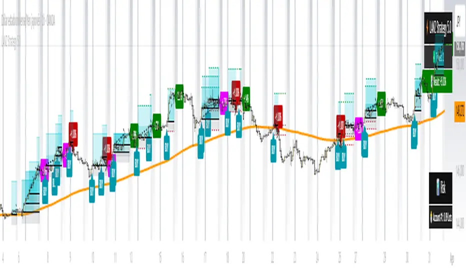
LANZ Strategy 6.0🔷 LANZ Strategy 6.0 — NY Session Entry Tool & Multi-Account Risk Manager
LANZ Strategy 6.0 - Is a trading tool designed to help traders plan, execute, and manage operations with a focus on risk management, multi-account handling, and visual clarity.
It works exclusively on the 1-hour timeframe ⏳ and is optimized for the New York market opening dynamics.
🧠 Core Concept
The strategy identifies bullish trading opportunities based on the 09:00 NY candle. Once detected, it automatically calculates and draws:
EP (Entry Price) — The exact level where the trade setup triggers.
SL (Stop Loss) — Based on a customizable percentage of the candle's high–low range or wick extremes.
TP (Take Profit) — Calculated using your chosen Risk–Reward Ratio (e.g., 1:5, 1:3, etc.).
⚙️ Main Features
⏳ Time-Specific Execution
Operates only when the 09:00 NY candle closes bullish.
Ideal for traders who align with the New York Session market structure.
💰 Multi-Account Lot Size Management
Up to 5 independent accounts can be configured with their own capital and risk %, showing the exact lot size to use for each.
📏 Adaptive Risk Control
Supports both Forex and non-Forex assets (indices, gold, oil).
For non-Forex, you can manually define the pip value according to your broker’s specs.
🎨 Visual Trade Map
Automatically plots clean and easy-to-read EP, SL, and TP lines with customizable colors, styles, and thickness.
A floating information panel displays levels, pip distances, and lot sizes.
🔔 Real-Time Alerts
Alerts for:
Entry signal detection.
Stop Loss hit.
Take Profit hit.
Manual close at the defined session end.
📊 Example
If you trade GBPUSD with Account #1 set to $10,000 and 2% risk,
and the 09:00 NY candle closes bullish with SL = 30 pips and RR = 5:1:
EP, SL, and TP levels are drawn instantly.
Risk = $200 (2% of $10,000).
Lot size is calculated automatically.
All details are shown in the on-chart panel.
🛠️ How to Use
Load the indicator on a 1-hour chart.
Configure risk settings and account data.
Wait for the 09:00 NY candle to close bullish.
Use the displayed lot size and levels to execute your trade.
Let the tool alert you for SL, TP, or manual close.
⚠️ Disclaimer:
This script is for educational purposes only. It does not guarantee profits and past performance does not represent future results. Always manage your risk responsibly.
👨💻 Credits:
💡 Developed by: LANZ
🧠 Execution Model & Logic Design: LANZ
📅 Designed for: 1H timeframe and NY-based entries

LANZ Strategy 7.0🔷 LANZ Strategy 7.0 — Multi-Session Breakout Logic with Midnight-Cross Support, Dynamic SL/TP, Multi-Account Lot Sizing & Real-Time Visual Tracking
LANZ Strategy 7.0 is a robust, visually-driven trading indicator designed to capture high-probability breakouts from a customizable market session.
It includes full support for sessions that cross midnight, dynamic calculation of Entry Price (EP), Stop Loss (SL) and Take Profit (TP) levels, and a multi-account lot sizing panel for precise risk management.
The system is built to only trigger one trade per day and manages the full trade lifecycle with automated visual cleanup and detailed alerts.
📌 This is an indicator, not a strategy — it does not place trades automatically, but provides exact entry setups, SL/TP levels, risk-based lot size guidance, and real-time alerts for execution.
🧠 Core Logic & Features
🚀 Entry Signal (BUY/SELL)
The trading day begins with a Decision Session (yellow box) where the high/low range is recorded.
Once the Operative Session starts (blue zone), the first touch of the session’s high triggers a BUY setup, and the first touch of the session’s low triggers a SELL setup.
Only one valid trade can be triggered per day — the system locks after the first signal.
⚙️ Dynamic Stop Loss & Take Profit
SL levels are derived from the Decision Session high/low using customizable Fibonacci multipliers (independent for BUY and SELL).
TP is dynamically calculated from the EP–SL distance using a user-defined Risk:Reward ratio (R:R).
All EP, SL, and TP levels are drawn as independent lines with customizable colors, label text size, and style.
⏳ Session & Midnight-Cross Support
Works with any custom Decision/Operative session hours, including sessions that start one day and end the next.
Properly tracks time zones using New York session time for consistency.
Includes Cutoff Time: after this limit, no new entries are allowed, and all visuals are auto-cleared if no trade was triggered.
💰 Multi-Account Risk-Based Lot Sizing
Supports up to 5 independent accounts.
Each account can have:
Own capital
Own risk percentage per trade
Lot size is auto-calculated based on:
SL distance (in pips or points)
Pip value (auto-detected for Forex or manually set for indices/commodities)
Results are displayed in a clean lot size info panel.
🖼️ Real-Time Visual Tracking
Dynamic updates to all levels during the Decision Session.
EP, SL, TP lines update if the session high/low changes before the Operative Session starts.
Trade result labels:
SL hit → “–1.00%” in red
TP hit → “+X.XX%” in green
Manual close at Operative End → shows actual % result in blue or purple.
🔔 Alerts for Every Key Event
Session start notification
EP entry triggered
SL or TP hit
Manual close at session end
Missed entry due to cutoff
🧭 Execution Flow
Decision Session (Yellow) — Capture high/low range.
Operative Session (Blue) — First touch of high = BUY setup; first touch of low = SELL setup.
Plot EP, SL, TP lines + calculate lot sizes for all active accounts.
Track trade until SL, TP, or Operative End.
If no entry triggered by Cutoff Time → clean all visuals and notify.
💡 Ideal For:
Traders who operate breakout logic on specific sessions (NY, London, Asian, or custom).
Those managing multiple accounts with strict risk per trade.
Anyone trading assets with sessions crossing midnight.
👨💻 Credits:
Developer: LANZ
Logic Design: LANZ
Built For: Multi-timeframe session breakouts with high precision.
Purpose: One-shot trade per day, risk consistency, and total visual clarity.
StratNinjaTableAuthor’s Instructions for StratNinjaTable
Purpose:
This indicator is designed to provide traders with a clear and dynamic table displaying The Strat candle patterns across multiple timeframes of your choice.
Usage:
Use the input panel to select which timeframes you want to monitor in the table.
Choose the table position on the chart (top left, center, right, or bottom).
The table will update each bar, showing the candle type, direction arrow, and remaining time until the candle closes for each selected timeframe.
Hover over or inspect the table to understand current market structure per timeframe using The Strat methodology.
Notes:
The Strat pattern is displayed as "1", "2U", "2D", or "3" based on the relationship of current and previous candle highs and lows.
The timer updates in real-time and adapts to daily, weekly, monthly, and extended timeframes.
This script requires Pine Script version 6. Please use it on supported platforms.
MFI or other indicators are not included in this base version but can be integrated separately if desired.
Credits:
Developed and inspired by shayy110 — thanks for your foundational work on The Strat in Pine Script.
Disclaimer:
This script is for educational and informational purposes only. Always verify signals and manage risk accordingly.

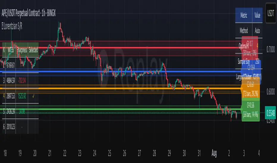
Lorentzian Key Support and Resistance Level Detector [mishy]🧮 Lorentzian Key S/R Levels Detector
Advanced Support & Resistance Detection Using Mathematical Clustering
The Problem
Traditional S/R indicators fail because they're either subjective (manual lines), rigid (fixed pivots), or break when price spikes occur. Most importantly, they don't tell you where prices actually spend time, just where they touched briefly.
The Solution: Lorentzian Distance Clustering
This indicator introduces a novel approach by using Lorentzian distance instead of traditional Euclidean distance for clustering. This is groundbreaking for financial data analysis.
Data Points Clustering:
🔬 Why Euclidean Distance Fails in Trading
Traditional K-means uses Euclidean distance:
• Formula: distance = (price_A - price_B)²
• Problem: Squaring amplifies differences exponentially
• Real impact: One 5% price spike has 25x more influence than a 1% move
• Result: Clusters get pulled toward outliers, missing real support/resistance zones
Example scenario:
Prices: ← flash spike
Euclidean: Centroid gets dragged toward 150
Actual S/R zone: Around 100 (where prices actually trade)
⚡ Lorentzian Distance: The Game Changer
Our approach uses Lorentzian distance:
• Formula: distance = log(1 + (price_difference)² / σ²)
• Breakthrough: Logarithmic compression keeps outliers in check
• Real impact: Large moves still matter, but don't dominate
• Result: Clusters focus on where prices actually spend time
Same example with Lorentzian:
Prices: ← flash spike
Lorentzian: Centroid stays near 100 (real trading zone)
Outlier (150): Acknowledged but not dominant
🧠 Adaptive Intelligence
The σ parameter isn't fixed,it's calculated from market disturbance/entropy:
• High volatility: σ increases, making algorithm more tolerant of large moves
• Low volatility: σ decreases, making algorithm more sensitive to small changes
• Self-calibrating: Adapts to any instrument or market condition automatically
Why this matters: Traditional methods treat a 2% move the same whether it's in a calm or volatile market. Lorentzian adapts the sensitivity based on current market behavior.
🎯 Automatic K-Selection (Elbow Method)
Instead of guessing how many S/R levels to draw, the indicator:
• Tests 2-6 clusters and calculates WCSS (tightness measure)
• Finds the "elbow" - where adding more clusters stops helping much
• Uses sharpness calculation to pick the optimal number automatically
Result: Perfect balance between detail and clarity.
How It Works
1. Collect recent closing prices
2. Calculate entropy to adapt to current market volatility
3. Cluster prices using Lorentzian K-means algorithm
4. Auto-select optimal cluster count via statistical analysis
5. Draw levels at cluster centers with deviation bands
📊 Manual K-Selection Guide (Using WCSS & Sharpness Analysis)
When you disable auto-selection, use both WCSS and Sharpness metrics from the analysis table to choose manually:
What WCSS tells you:
• Lower WCSS = tighter clusters = better S/R levels
• Higher WCSS = scattered clusters = weaker levels
What Sharpness tells you:
• Higher positive values = optimal elbow point = best K choice
• Lower/negative values = poor elbow definition = avoid this K
• Measures the "sharpness" of the WCSS curve drop-off
Decision strategy using both metrics:
K=2: WCSS = 150.42 | Sharpness = - | Selected =
K=3: WCSS = 89.15 | Sharpness = 22.04 | Selected = ✓ ← Best choice
K=4: WCSS = 76.23 | Sharpness = 1.89 | Selected =
K=5: WCSS = 73.91 | Sharpness = 1.43 | Selected =
Quick decision rules:
• Pick K with highest positive Sharpness (indicates optimal elbow)
• Confirm with significant WCSS drop (30%+ reduction is good)
• Avoid K values with negative or very low Sharpness (<1.0)
• K=3 above shows: Big WCSS drop (41%) + High Sharpness (22.04) = Perfect choice
Why this works:
The algorithm finds the "elbow" where adding more clusters stops being useful. High Sharpness pinpoints this elbow mathematically, while WCSS confirms the clustering quality.
Elbow Method Visualization:
Traditional clustering problems:
❌ Price spikes distort results
❌ Fixed parameters don't adapt
❌ Manual tuning is subjective
❌ No way to validate choices
Lorentzian solution:
☑️ Outlier-resistant distance metric
☑️ Entropy-based adaptation to volatility
☑️ Automatic optimal K selection
☑️ Statistical validation via WCSS & Sharpness
Features
Visual:
• Color-coded levels (red=highest resistance, green=lowest support)
• Optional deviation bands showing cluster spread
• Strength scores on labels: Each cluster shows a reliability score.
• Higher scores (0.8+) = very strong S/R levels with tight price clustering
• Lower scores (0.6-0.7) = weaker levels, use with caution
• Based on cluster tightness and data point density
• Clean line extensions and labels
Analytics:
• WCSS analysis table showing why K was chosen
• Cluster metrics and statistics
• Real-time entropy monitoring
Control:
• Auto/manual K selection toggle
• Customizable sample size (20-500 bars)
• Show/hide bands and metrics tables
The Result
You get mathematically validated S/R levels that focus on where prices actually cluster, not where they randomly spiked. The algorithm adapts to market conditions and removes guesswork from level selection.
Best for: Traders who want objective, data-driven S/R levels without manual chart analysis.
Credits: This script is for educational purposes and is inspired by the work of @ThinkLogicAI and an amazing mentor @DskyzInvestments . It demonstrates how Lorentzian geometrical concepts can be applied not only in ML classification but also quite elegantly in clustering.
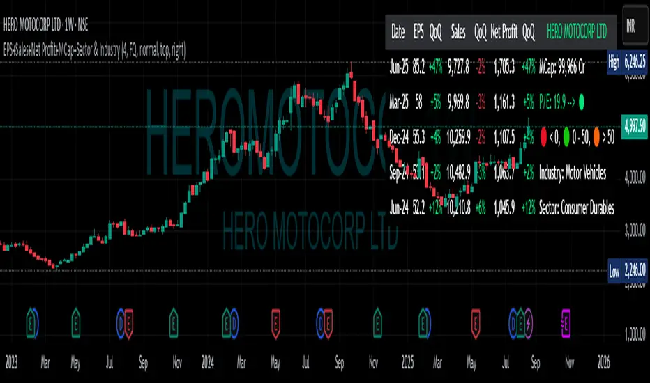
EPS+Sales+Net Profit+MCap+Sector & Industry📄 Full Description
This script displays a comprehensive financial data panel directly on your TradingView chart, helping long-term investors and swing traders make informed decisions based on fundamental trends. It consolidates key financial metrics and business classification data into a single, visually clear table.
🔍 Key Features:
🧾 Financial Metrics (Auto-Fetched via request.financial):
EPS (Earnings Per Share) – Displayed with trend direction (QoQ or YoY).
Sales / Revenue – In ₹ Crores (for Indian stocks), trend change also included.
Net Profit – Also in ₹ Crores, along with percentage change.
Market Cap – Automatically calculated using outstanding shares × price, shown in ₹ Cr.
Free Float Market Cap – Based on float shares × price, also in ₹ Cr.
🏷️ Sector & Industry Info:
Automatically identifies and displays the Sector and Industry of the stock using syminfo.sector and syminfo.industry.
Displayed inline with metrics, making it easy to know what business the stock belongs to.
📊 Table View:
Compact and responsive table shown on your chart.
Columns: Date | EPS | QoQ | Sales | QoQ | Net Profit | QoQ | Metrics
Metrics column dynamically shows:
Market Cap
Free Float
Sector (Row 4)
Industry (Row 5)
🌗 Appearance:
Supports Dark Mode and Mini Mode toggle.
You can also customize:
Number of data points (last 4+ quarters or years)
Table position and size
🎯 Use Case:
This script is ideal for:
Fundamental-focused traders who use EPS/Sales trends to identify momentum.
Swing traders who combine price action with fundamental tailwinds.
Portfolio builders who want to see sector/industry alignment quickly.
It works best with fundamentally sound stocks where earnings and profitability are a major factor in price movements.
✅ Important Notes:
Script uses request.financial which only works with supported symbols (mostly stocks).
Market Cap and Free Float are calculated in ₹ Crores.
All financial values are rounded and formatted for readability (e.g., 1,234 Cr).
🙏 Credits:
Developed and published by Sameer Thorappa
Built with a clean, minimalist approach for high readability and functionality.
Trend Buy/Sell Fibonacci Range - KLTThe Trend Buy/Sell Fibonacci Range – KLT indicator identifies bullish and bearish trends based on where the closing price is located within a Fibonacci range calculated from the last N candles (default is 10). Instead of analyzing individual candles, this tool takes a broader view of price action using Fibonacci retracement levels across a dynamic multi-candle range.
How It Works:
Range Calculation
The indicator calculates the highest high and lowest low over the last N candles to define the active price range (default: 10 bars).
Fibonacci Levels
Within this range, Fibonacci levels (0.236, 0.382, 0.5, 0.618, 0.786) are dynamically computed. These levels act as internal thresholds to evaluate bullish or bearish pressure.
Trend Identification (via Close Position):
If the closing price is above the 0.618 level, it indicates strong buy pressure → the candle turns green and an upward triangle appears.
If the closing price is below the 0.382 level, it suggests strong sell pressure → the candle turns red and a downward triangle is displayed.
If the close lies between 0.382 and 0.618, the market is considered neutral, and the candle is gray.
Visual Elements:
Colored candles to immediately spot trend conditions.
Triangle signals (optional) for clear Buy/Sell markers.
Fibonacci level lines plotted on the chart for full context (can be toggled on/off).
Customization Options:
Lookback period (number of candles to calculate the range)
Fibonacci threshold levels (upper/lower)
Show/hide arrows and Fibonacci lines
Why Use This Indicator?
This tool is perfect for traders who want a simple visual method to assess trend strength based on price structure, not indicators derived from lagging moving averages. It offers:
Cleaner market structure analysis
Objective trend zones
Customizable sensitivity
Recommended Use:
Works well in conjunction with support/resistance zones, volume, or momentum indicators.
Applicable to any asset class or timeframe.
Credits:
Developed by KLT, combining structure-based logic with Fibonacci precision.

LANZ Strategy 6.0 [Backtest]🔷 LANZ Strategy 6.0 — Precision Backtesting Based on 09:00 NY Candle, Dynamic SL/TP, and Lot Size per Trade
LANZ Strategy 6.0 is the simulation version of the original LANZ 6.0 indicator. It executes a single LIMIT BUY order per day based on the 09:00 a.m. New York candle, using dynamic Stop Loss and Take Profit levels derived from the candle range. Position sizing is calculated automatically using capital, risk percentage, and pip value — allowing accurate trade simulation and performance tracking.
📌 This is a strategy script — It simulates real trades using strategy.entry() and strategy.exit() with full money management for risk-based backtesting.
🧠 Core Logic & Trade Conditions
🔹 BUY Signal Trigger:
At 09:00 a.m. NY (New York time), if:
The current candle is bullish (close > open)
→ A BUY order is placed at the candle’s close price (EP)
Only one signal is evaluated per day.
⚙️ Stop Loss / Take Profit Logic
SL can be:
Wick low (0%)
Or dynamically calculated using a % of the full candle range
TP is calculated using the user-defined Risk/Reward ratio (e.g., 1:4)
The TP and SL levels are passed to strategy.exit() for each trade simulation.
💰 Risk Management & Lot Size Calculation
Before placing the trade:
The system calculates pip distance from EP to SL
Computes the lot size based on:
Account capital
Risk % per trade
Pip value (auto or manual)
This ensures every trade uses consistent, scalable risk regardless of instrument.
🕒 Manual Close at 3:00 p.m. NY
If the trade is still open by 15:00 NY time, it will be closed using strategy.close().
The final result is the actual % gain/loss based on how far price moved relative to SL.
📊 Backtest Accuracy
One trade per day
LIMIT order at the candle close
SL and TP pre-defined at execution
No repainting
Session-restricted (only runs on 1H timeframe)
✅ Ideal For:
Traders who want to backtest a clean and simple daily entry system
Strategy developers seeking reproducible, high-conviction trades
Users who prefer non-repainting, session-based simulations
👨💻 Credits:
💡 Developed by: LANZ
🧠 Logic & Money Management Engine: LANZ
📈 Designed for: 1H charts
🧪 Purpose: Accurate simulation of LANZ 6.0's NY Candle Entry system

LANZ Strategy 5.0 [Backtest]🔷 LANZ Strategy 5.0 — Rule-Based BUY Logic with Time Filter, Session Limits and Auto SL/TP Execution
This is the backtest version of LANZ Strategy 5.0, built as a strategy script to evaluate real performance under fixed intraday conditions. It automatically places BUY and SELL trades based on structured candle confirmation, EMA trend alignment, and session-based filters. The system simulates real-time execution with precise Stop Loss and Take Profit levels.
📌 Built for traders seeking to simulate clean intraday logic with fully automated entries and performance metrics.
🧠 Core Logic & Strategy Conditions
✅ BUY Signal Conditions:
Price is above the EMA200
The last 3 candles are bullish (close > open)
The signal occurs within the defined session window (NY time)
Daily trade limit has not been exceeded
If all are true, a BUY order is executed at market, with SL and TP set immediately.
🔻 SELL Signal Conditions (Optional):
Exactly inverse to BUY (below EMA + 3 bearish candles). Disabled by default.
🕐 Operational Time Filter (New York Time)
You can fully customize your intraday window:
Start Time: e.g., 01:15 NY
End Time: e.g., 16:00 NY
The system evaluates signals only within this range, even across midnight if configured.
🔁 Trade Management System
One trade at a time per signal
Trades include a Stop Loss (SL) and Take Profit (TP) based on pip distance
Trade result is calculated automatically
Each signal is shown with a triangle marker (BUY only, by default)
🧪 Backtest Accuracy
This version uses:
strategy.order() for entries
strategy.exit() for SL and TP
strategy.close_all() at the configured manual closing time
This ensures realistic behavior in the TradingView strategy tester.
⚙️ Flow Summary (Step-by-Step)
On every bar, check:
Is the time within the operational session?
Is the price above the EMA?
Are the last 3 candles bullish?
If conditions met → A BUY trade is opened:
SL = entry – X pips
TP = entry + Y pips
Trade closes:
If SL or TP is hit
Or at the configured manual close time (e.g., 16:00 NY)
📊 Settings Overview
Timeframe: 1-hour (ideal)
SL/TP: Configurable in pips
Max trades/day: User-defined (default = 99 = unlimited)
Manual close: Adjustable by time
Entry type: Market (not limit)
Visuals: Plotshape triangle for BUY entry
👨💻 Credits:
💡 Developed by: LANZ
🧠 Strategy logic & execution: LANZ
✅ Designed for: Clean backtesting, clarity in execution, and intraday logic simulation

LANZ Strategy 5.0🔷 LANZ Strategy 5.0 — Intraday BUY Signals, Dynamic Lot Size per Account, Real-Time Dashboard and Smart Execution
LANZ Strategy 5.0 is a powerful intraday tool designed for traders who need a visual-first, data-backed BUY system, enhanced with risk-aware lot size calculation and a real-time performance dashboard. This indicator intelligently detects strong momentum setups and provides visual and statistical clarity throughout the session.
📌 This is an indicator, not a strategy — It does not place trades automatically but provides precise conditions, alerts, and visual guides to support execution.
🧠 Core Logic & Features
BUY Entry Conditions (Signal Engine)
A BUY signal is triggered when:
The current price is above the EMA200 (trend filter)
The last 3 candles are bullish (candle body close > open)
You are within the defined session window (NY time)
When all conditions are met and you haven’t reached the daily trade limit, a signal appears on the chart and an optional alert is triggered.
Operational Hours Filter (NY Time)
You define:
Start time (e.g., 01:15 NY)
End time (e.g., 16:00 NY)
The system only evaluates and executes signals within this period. If a BUY setup occurs outside the window, it’s ignored. The chart is also highlighted with a transparent teal background to visually show active trading hours.
Lot Size Panel with Per-Account Risk Management
Designed for traders managing multiple accounts or capital sources. You can enable up to 5 accounts, each with:
Its own capital
Its own risk percentage per trade
The system uses the defined SL in pips, plus the instrument’s pip value, to calculate the lot size per account. All values are shown in a dedicated panel at the bottom-right, automatically updating with each new trade.
The emojis (🐣🦊🦁🐲🐳) distinguish each account visually.
Trade Visualization with Customizable Lines
When a signal is triggered:
An Entry Point (EP) line is drawn at the candle’s close.
A Stop Loss (SL) line is placed X pips below the entry.
A Take Profit (TP) line is placed Y pips above the entry.
All three lines are fully customizable in style, color, and thickness. You define how many bars the lines should extend.
Outcome Tracking & Real-Time Dashboard
Each trade outcome is measured:
SL hit = –1.00%
TP hit = +3.00%
Manual close = calculated dynamically based on price at close time
Each result is labeled on the chart near its level, and stored.
The top-right dashboard updates in real time:
✅ Number of trades
📈 Cumulative % gain/loss of the day (color-coded)
Alerts You Can Trust:
You’ll get a Buy Alert when a valid signal is formed
You’ll get a Trade Executed Alert when the visual operation is plotted
You’ll get a SL/TP Hit Alert with price and result
You’ll get a Manual Close Alert if the configured time is reached and the trade is still active
⚙️ Step-by-Step Execution Flow
At every bar, the system checks:
Are we within the session time window?
Is price above EMA?
Are the last 3 candles bullish?
✅ If yes:
A BUY signal is plotted
Entry/SL/TP lines are drawn
Lot sizes are calculated and displayed
Trade is added to the daily count
🕐 At the configured Manual Close time (e.g., 16:00 NY):
If the trade is still open, it's closed
A label is added with the exact result in %
💡 Ideal For:
Intraday traders who operate within fixed time sessions
Traders managing multiple accounts or capital pools
Anyone who wants full visual clarity of every decision point
Traders who appreciate dynamic lot size calculation and clean execution tracking
👨💻 Credits:
💡 Developed by: LANZ
🧠 Strategy concept & execution model: LANZ
🧪 Tested on: 1H charts with visual-only execution
📈 Designed for: Clarity, adaptability, and full intraday control
3D Surface Modeling [PhenLabs]📊 3D Surface Modeling
Version: PineScript™ v6
📌 Description
The 3D Surface Modeling indicator revolutionizes technical analysis by generating three-dimensional visualizations of multiple technical indicators across various timeframes. This advanced analytical tool processes and renders complex indicator data through a sophisticated matrix-based calculation system, creating an intuitive 3D surface representation of market dynamics.
The indicator employs array-based computations to simultaneously analyze multiple instances of selected technical indicators, mapping their behavior patterns across different temporal dimensions. This unique approach enables traders to identify complex market patterns and relationships that may be invisible in traditional 2D charts.
🚀 Points of Innovation
Matrix-Based Computation Engine: Processes up to 500 concurrent indicator calculations in real-time
Dynamic 3D Rendering System: Creates depth perception through sophisticated line arrays and color gradients
Multi-Indicator Integration: Seamlessly combines VWAP, Hurst, RSI, Stochastic, CCI, MFI, and Fractal Dimension analyses
Adaptive Scaling Algorithm: Automatically adjusts visualization parameters based on indicator type and market conditions
🔧 Core Components
Indicator Processing Module: Handles real-time calculation of multiple technical indicators using array-based mathematics
3D Visualization Engine: Converts indicator data into three-dimensional surfaces using line arrays and color mapping
Dynamic Scaling System: Implements custom normalization algorithms for different indicator types
Color Gradient Generator: Creates depth perception through programmatic color transitions
🔥 Key Features
Multi-Indicator Support: Comprehensive analysis across seven different technical indicators
Customizable Visualization: User-defined color schemes and line width parameters
Real-time Processing: Continuous calculation and rendering of 3D surfaces
Cross-Timeframe Analysis: Simultaneous visualization of indicator behavior across multiple periods
🎨 Visualization
Surface Plot: Three-dimensional representation using up to 500 lines with dynamic color gradients
Depth Indicators: Color intensity variations showing indicator value magnitude
Pattern Recognition: Visual identification of market structures across multiple timeframes
📖 Usage Guidelines
Indicator Selection
Type: VWAP, Hurst, RSI, Stochastic, CCI, MFI, Fractal Dimension
Default: VWAP
Starting Length: Minimum 5 periods
Default: 10
Step Size: Interval between calculations
Range: 1-10
Visualization Parameters
Color Scheme: Green, Red, Blue options
Line Width: 1-5 pixels
Surface Resolution: Up to 500 lines
✅ Best Use Cases
Multi-timeframe market analysis
Pattern recognition across different technical indicators
Trend strength assessment through 3D visualization
Market behavior study across multiple periods
⚠️ Limitations
High computational resource requirements
Maximum 500 line restriction
Requires substantial historical data
Complex visualization learning curve
🔬 How It Works
1. Data Processing:
Calculates selected indicator values across multiple timeframes
Stores results in multi-dimensional arrays
Applies custom scaling algorithms
2. Visualization Generation:
Creates line arrays for 3D surface representation
Applies color gradients based on value magnitude
Renders real-time updates to surface plot
3. Display Integration:
Synchronizes with chart timeframe
Updates surface plot dynamically
Maintains visual consistency across updates
🌟 Credits:
Inspired by LonesomeTheBlue (modified for multiple indicator types with scaling fixes and additional unique mappings)
💡 Note:
Optimal performance requires sufficient computing resources and historical data. Users should start with default settings and gradually adjust parameters based on their analysis requirements and system capabilities.

Initial Balance Wave MapThis indicator visualizes the Initial Balance (IB) range for any session, marking the first hour's high and low. It includes optional midpoints, extensions (e.g. 1.5x IB, 2x IB), and customizable time windows. Additional features allow users to display session open, high, low, close, and VWAP reference points. Designed to support price action and session structure analysis, it adapts to various global futures and FX market opens. All display elements are optional and fully configurable.
This updated indicator builds upon the open-source foundation by @noop-noop with enhancements and user-facing labels tailored for Auction Market Theory, scalping, and structure-based trade setups.
Key updated Featured: Multiple previous day's IB levels carry forward into the current day's chart, as opposed to just the previous day's levels carrying forward to the new IB time.
🙌 Credits:
This script builds upon the excellent open-source work by @noop-noop. Original script available here .

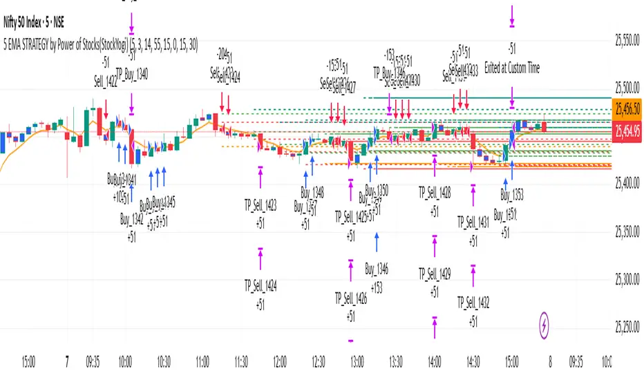
5 EMA STRATEGY by Power of Stocks(StockYogi)5 EMA STRATEGY by Power of Stocks(StockYogi)
This is a 5 EMA Breakout Strategy inspired by the trading principles taught by Shubhashi Pani, founder of the Power of Stocks (POS) community.
The strategy is designed to:
• Detect breakout setups when price breaks the high/low of a signal candle (based on EMA conditions)
• Enter trades only if the breakout occurs within the next 3 candles
• Allow multiple trades in the same direction without closing the earlier one
• Use independent stop-loss (SL) and take-profit (TP) targets for each trade based on a user-defined risk-reward ratio
• Optionally enter trades only at candle close
• Optionally avoid trades during a custom time window (e.g., 3:00 PM to 3:30 PM IST)
• Optionally close all open positions at a defined time (e.g., 3:30 PM IST)
The goal of this strategy is to provide greater flexibility and realism for intraday or short-term traders following structured breakout systems.
Disclaimer: This script is an implementation of technical ideas for educational purposes only. It is not financial advice. All trading involves risk, and past performance does not guarantee future results.
Strategy Credits:
This strategy is based on publicly known breakout rules taught by Shubhashi Pani (Power of Stocks). This is not an official POS script, and I am not affiliated with the Power of Stocks team. This implementation was developed independently to follow the logic shared for educational use.
Feel free to use, backtest, and modify according to your needs. Constructive feedback is welcome!
LANZ Strategy 1.0 [Backtest]🔷 LANZ Strategy 1.0 — Time-Based Session Trading with Smart Reversal Logic and Risk-Controlled Limit Orders
This backtest version of LANZ Strategy 1.0 brings precision to session-based trading by using directional confirmation, pre-defined risk parameters, and limit orders that execute overnight. Designed for the 1-hour timeframe, it allows traders to evaluate the system with configurable SL, TP, and risk settings in a fully automated environment.
🧠 Core Strategy Logic:
1. Directional Confirmation at 18:00 NY:
At 18:00 NY, the system compares the 08:00 open vs the 18:00 close:
If the direction matches the previous day, the signal is reversed.
If the direction differs, the current day's trend is kept.
This logic is designed to avoid momentum exhaustion and capture corrective reversals.
2. Entry Level Definition:
Based on the confirmed direction:
For BUY, the Low of the day is used as Entry Point (EP).
For SELL, the High of the day becomes EP.
The system plots a Stop Loss and Take Profit based on user-defined pip inputs (default: SL = 18 pips, TP = 54 pips → RR 1:3).
3. Time-Limited Entry Execution (LIMIT Orders):
Orders are sent after 18:00 NY and can be triggered anytime between 18:00 and 08:00 NY.
If EP is not touched before 08:00, the order is automatically cancelled.
4. Manual Close Feature:
If the trade is still open at the configured hour (default 09:00 NY), the system closes all positions, simulating realistic intraday exit scenarios.
5. Lot Size Calculation Based on Risk:
Lot size is dynamically calculated using the account size, risk percentage, and SL distance.
This ensures consistent risk exposure regardless of market volatility.
⚙️ Step-by-Step Flow:
08:00 NY → Captures the open of the day.
18:00 NY → Confirms direction and defines EP, SL, and TP.
After 18:00 NY → If conditions are met, a LIMIT order is placed at EP.
Between 18:00–08:00 NY → If price touches EP, the trade is executed.
At 08:00 NY → If EP wasn’t touched, the order is cancelled.
At Configured Manual Close Time (default 09:00 NY) → All open positions are force-closed if still active.
🧪 Backtest Settings:
Timeframe: 1-hour only
Order Type: strategy.entry() with limit=
SL/TP Configurable: Yes, in pips
Risk Input: % of capital per trade
Manual Close Time: Fully adjustable (default 09:00 NY)
👨💻 Credits:
Developed by LANZ
Strategy logic and trading concept built with clarity and precision.
Code structure and documentation by Kairos, your AI trading assistant.
Designed for high-confidence execution and clean backtesting performance.

LANZ Strategy 1.0🔷 LANZ Strategy 1.0 — Session-Based Directional Logic with Visual Multi-Account Risk Management
LANZ Strategy 1.0 is a structured and disciplined trading strategy designed for the 1-hour timeframe, operating during the NY session and executing trades overnight. It uses the directional behavior between 08:00 and 18:00 New York time to define precise limit entries for the following night. Ideal for traders who prefer time-based execution, clear visuals, and professional risk management across multiple accounts.
🧠 Core Components:
1. Session Direction Confirmation:
At 18:00 NY, the system evaluates the market direction by comparing the open at 08:00 vs the close at 18:00:
If the direction matches the previous day, it is reversed.
If it differs, the current day’s direction is kept.
This logic is designed to avoid trend exhaustion and favor potential reversal opportunities.
2. EP Level & Risk Definition:
Once direction is defined:
For BUY, EP is set at the Low of the session.
For SELL, EP is set at the High of the session.
The system automatically plots:
SL fixed at 18 pips from EP
TP at 3.00× the risk → 54 pips from EP
All levels (EP, SL, TP) are shown with visual lines and price labels.
3. Time-Restricted Entry Execution:
The entry is only valid if price touches the EP between 19:00 and 08:00 NY.
If EP is not touched before 08:00 NY, the trade is automatically cancelled.
4. Multi-Account Lot Sizing:
Traders can configure up to five different accounts, each with its own capital and risk percentage.
The system calculates and displays the lot size per account, based on SL distance and pip value, in a dynamic floating label.
5. Outcome Tracking:
If TP is hit, a +3.00% profit label is displayed along with a congratulatory alert.
If SL is hit, a -1.00% label appears with a loss alert.
If the trade is still open by 09:00 NY, it is manually closed, and the result is shown as a percentage of the initial risk.
📊 Visual Features:
Custom-colored angle and guide lines.
Dynamic angle line starts at 08:00 NY and tracks price until 18:00.
Shaded backgrounds for key time zones (e.g., 08:00, 18:00, 19:00).
BUY/SELL signals shown at 19:00 based on match/divergence logic.
Label panel showing risk metrics and lot size for each active account.
⚙️ How It Works:
08:00 NY: Marks the session open and initiates a dynamic angle line.
18:00 NY: Evaluates the session direction and calculates EP/SL/TP based on outcome.
19:00 NY: Activates limit order monitoring.
During the night (until 08:00 NY): If EP is touched, the trade is triggered.
At 08:00 NY: If no touch occurred, trade is cancelled.
Overnight: TP/SL logic is enforced, showing percentage outcomes.
At 09:00 NY: If still open, trade is closed manually and result is labeled visually.
🔔 Alerts:
🚀 EP execution alert when touched
💢 Stop Loss hit alert
⚡ Take Profit hit alert
✅ Manual close at 09:00 NY with performance result
🔔 Daily reminder at 19:00 NY to configure and prepare the trade
📝 Notes:
Strategy is exclusive to the 1-hour timeframe.
Works best on assets with clean NY session movement.
Perfect for structured, semi-automated swing/overnight trading styles.
Fully visual, self-explanatory, and backtest-friendly.
👨💻 Credits:
Developed by LANZ
A strategy created with precision, discipline, and a vision for traders who value time-based entries, clean execution logic, and visual confidence on the chart.
Special thanks to Kairos — your AI assistant — for the detailed structure, scripting, and documentation of the strategy.
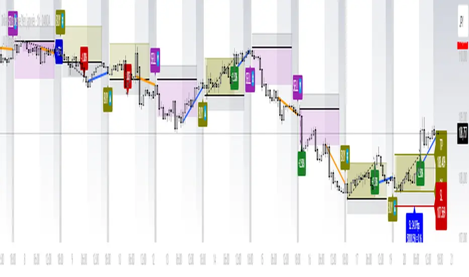
SOT & SA Detector ProSOT & SA Detector Pro- Advanced Reversal Pattern Recognition
OVERVIEW
The SOT & SA Detector is an educational indicator designed to identify potential market reversal points through systematic analysis of candlestick patterns, volume confirmation, and price wave structures. SOT (Shorting of Thrust) signals suggest potential bearish reversals after upward price movements, while SA (Selling Accumulation) signals indicate possible bullish reversals following downward trends. This tool helps traders recognize key market transition points by combining multiple technical criteria for enhanced signal reliability.
═══════════════════════════════════════════════════════════════
HOW IT WORKS
Technical Methodology
The indicator employs a multi-factor analysis approach that evaluates:
Wave Structure Analysis: Identifies minimum 2-bar directional waves (upward for SOT, downward for SA)
Price Delta Validation: Ensures closing price changes remain within specified percentage thresholds (default 0.3%) best 0.1.
Candlestick Tail Analysis: Measures rejection wicks using configurable tail multipliers
Volume Confirmation: Requires increased volume compared to previous periods
Pattern Confirmation: Validates signals through subsequent price action
Signal Generation Process
Pattern Recognition: Scans for qualifying candlestick formations with appropriate tail characteristics
Volume Verification: Confirms patterns with volume expansion using adjustable multiplier
Price Confirmation: Validates signals when price breaks and closes beyond pattern extremes
Signal Display: Places labeled markers and draws horizontal reference levels
Mathematical Foundation
Delta calculation: math.abs(close - close ) / close <= deltaPercent / 100
Tail analysis: (high - close ) >= tailMultiplier * (close - low ) for SOT
Volume filter: volume >= volume * volumeFactor
═══════════════════════════════════════════════════════════════
KEY FEATURES
Dual Pattern Recognition: Identifies both bullish (SA) and bearish (SOT) reversal candidates
Volume Integration: Incorporates volume analysis for enhanced signal validation
Customizable Parameters: Adjustable wave length, delta percentage, tail multiplier, and volume factor
Visual Clarity: Color-coded bar highlighting, labeled signals, and horizontal reference levels
Time-Based Filtering: Configurable analysis period to focus on recent market activity
Non-Repainting Signals: Confirmed signals remain stable and do not change with new price data
Alert System: Built-in notifications for both initial signals and subsequent confirmations
═══════════════════════════════════════════════════════════════
HOW TO USE
Signal Interpretation
Red SOT Labels: Appear above potential bearish reversal candles with downward-pointing markers
Green SA Labels: Display below potential bullish reversal candles with upward-pointing markers
Horizontal Lines: Extend from signal levels to provide ongoing reference points
Bar Coloring: Highlights qualifying pattern candles for visual emphasis
Trading Application
This indicator serves as an educational tool for pattern recognition and should be used in conjunction with additional analysis methods. Consider SOT signals as potential areas of selling pressure following upward moves, while SA signals may indicate buying interest after downward price action.
Best Practices
Combine with trend analysis and support/resistance levels
Consider overall market context and timeframe alignment
Use proper risk management techniques
Validate signals with additional technical indicators
═══════════════════════════════════════════════════════════════
SETTINGS
Analysis Days (Default: 20)
Controls the lookback period for signal detection. Higher values extend historical analysis while lower values focus on recent activity.
Minimum Bars in Wave (Default: 2)
Sets the minimum consecutive bars required to establish directional wave patterns. Increase for stronger trend confirmation.
Max Close Change % (Default: 0.3) best 0.1.
Defines acceptable closing price variation between consecutive bars. Lower values require tighter price consolidation.
Tail Multiplier (Default: 1.0) best 1.5 or more.
Adjusts sensitivity for candlestick tail analysis. Higher values require more pronounced rejection wicks.
Volume Factor (Default: 1.0)
Sets volume expansion threshold compared to previous period. Values above 1.0 require volume increases.
═══════════════════════════════════════════════════════════════
LIMITATIONS
Market Conditions
May produce false signals in highly volatile or low-volume conditions
Effectiveness varies across different market environments and timeframes
Requires sufficient volume data for optimal performance
Signal Timing
Signals appear after pattern completion, not in real-time during formation
Confirmation signals depend on subsequent price action
Historical signals do not guarantee future market behavior
Technical Constraints
Limited to analyzing price and volume data only
Does not incorporate fundamental analysis or external market factors
Performance may vary significantly across different trading instruments
═══════════════════════════════════════════════════════════════
IMPORTANT DISCLAIMERS
This indicator is designed for educational purposes and technical analysis learning. It does not constitute financial advice, investment recommendations, or trading signals. Past performance does not guarantee future results. Trading involves substantial risk of loss, and this tool should be used alongside proper risk management techniques and additional analysis methods.
Always conduct thorough analysis using multiple indicators and consider market context before making trading decisions. The SOT & SA patterns represent potential reversal points but do not guarantee price direction changes.
═══════════════════════════════════════════════════════════════
Credits: Original concept and Pine Script implementation by Everyday_Trader_X
Version: Pine Script v6 compatible
Category: Technical Analysis / Reversal Detection
Overlay: Yes (displays on price chart)
QG-Particle OscillatorThis is an advanced oscillator based on auxiliary particle filter. It separates signal from noise and uses smoothing algorithm similar to JMA.
The main oscillator line is a smoothed and detrended version of the price series similar to detrended oscillator line. The purple/aqua lines are a prediction based on an additional adaptive smoothing technique and current volatility.
The prediction is smoothed twice and is supposed to represent the true signal without any noise, thus the prediction should always be less than the raw detrend line. However, certain volatile conditions will cause the prediction to cross above/below the detrend line. When this happens the likelihood of a reversal or pullback is extremely high.
There are 3 dots on the zero line- Red, Green and Yellow. The yellow dots warn of an eminent pullback 2 bars before it actually occurs. This is a non-repainting indicator.
One can also use this indicator to trade CCI signals, similar to zero line rejection in existing trend.
The indicator has 2 settings- Period and Phase. The phase represents cycle phase and Period represents oscillator period.
Credits: This indicator has been originally published for Ninjatrader and this is conversion into pinescript.

LANZ Strategy 4.0 [Backtest]🔷 LANZ Strategy 4.0 — Strategy Execution Based on Confirmed Structure + Risk-Based SL/TP
LANZ Strategy 4.0 is the official backtesting engine for the LANZ Strategy 4.0 trading logic. It simulates real-time executions based on breakout of Strong/Weak Highs or Lows, using a consistent structural system with SL/TP dynamically calculated per trade. With integrated risk management and lot size logic, this script allows traders to validate LANZ Strategy 4.0 performance with real strategy metrics.
🧠 Core Components:
Confirmed Breakout Entries: Trades are executed only when price breaks the most recent structural level (Strong High or Strong Low), detected using swing pivots.
Dynamic SL and TP Logic: SL is placed below/above the breakout point with a customizable buffer. TP is defined using a fixed Risk-Reward (RR) ratio.
Capital-Based Risk Management: Lot size is calculated based on account equity, SL distance, and pip value (e.g. $10 per pip on XAUUSD).
Clean and Controlled Executions: Only one trade is active at a time. No new entries are allowed until the current position is closed.
📊 Visual Features:
Automatic plotting of Entry, SL, and TP levels.
Full control of swing sensitivity (swingLength) and SL buffer.
SL and TP lines extend visually for clarity of trade risk and reward zones.
⚙️ How It Works:
Detects pivots and classifies trend direction.
Waits for breakout above Strong High (BUY) or below Strong Low (SELL).
Calculates dynamic SL and TP based on buffer and RR.
Computes trade size automatically based on risk per trade %.
Executes entry and manages exits via strategy engine.
📝 Notes:
Ideal for evaluating the LANZ Strategy 4.0 logic over historical data.
Must be paired with the original indicator (LANZ Strategy 4.0) for live trading.
Best used on assets with clear structural behavior (gold, indices, FX).
📌 Credits:
Backtest engine developed by LANZ based on the official rules of LANZ Strategy 4.0. This script ensures visual and logical consistency between live charting and backtesting simulations.
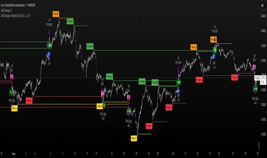
LANZ Strategy 3.0 [Backtest]🔷 LANZ Strategy 3.0 — Asian Range Fibonacci Scalping Strategy
LANZ Strategy 3.0 is a precision-engineered backtesting tool tailored for intraday traders who rely on the Asian session range to determine directional bias. This strategy implements dynamic Fibonacci projections and strict time-window validation to simulate a clean and disciplined trading environment.
🧠 Core Components:
Asian Range Bias Definition: Direction is established between 01:15–02:15 a.m. NY time based on the candle’s close in relation to the midpoint of the Asian session range (18:00–01:15 NY).
Limit Order Execution: Only one trade is placed daily, using a limit order at the Asian range high (for sells) or low (for buys), between 01:15–08:00 a.m. NY.
Fibonacci-Based TP/SL:
Original Mode: TP = 2.25x range, SL = 0.75x range.
Optimized Mode: TP = 1.95x range, SL = 0.65x range.
No Trade After 08:00 NY: If the limit order is not executed before 08:00 a.m. NY, it is canceled.
Fallback Logic at 02:15 NY: If the market direction misaligns with the setup at 02:15 a.m., the system re-evaluates and can re-issue the order.
End-of-Day Closure: All positions are closed at 15:45 NY if still open.
📊 Backtest-Ready Design:
Entries and exits are executed using strategy.entry() and strategy.exit() functions.
Position size is fixed via capital risk allocation ($100 per trade by default).
Only one position can be active at a time, ensuring controlled risk.
📝 Notes:
This strategy is ideal for assets sensitive to the Asian/London session overlap, such as Forex pairs and indices.
Easily switch between Fibonacci versions using a single dropdown input.
Fully deterministic: all entries are based on pre-defined conditions and time constraints.
👤 Credits:
Strategy developed by rau_u_lanz using Pine Script v6. Built for traders who favor clean sessions, directional clarity, and consistent execution using time-based logic and Fibonacci projections.

LANZ Strategy 2.0 [Backtest]🔷 LANZ Strategy 2.0 — Structural Breakout Logic with Dynamic Swing Protection
LANZ Strategy 2.0 is a precision-focused backtesting system built for intraday traders who rely on structural confirmations before the London session to guide directional bias. This tool uses smart swing detection, risk-defined position sizing, and strict time-based execution to simulate real trading conditions with clarity and control.
🧠 Core Components:
Structural Confirmation (Trend & BoS): Detects trend direction and break of structure (BoS) using a three-swing logic, aligning trade entries with valid structural movement.
Time-Based Execution: Trades are triggered exclusively at 02:00 a.m. New York time, ensuring disciplined and repeatable intraday testing.
Swing-Based SL Models: Traders can select between three stop-loss protection types:
First Swing: Most recent structural level
Second Swing: Prior level
Full Coverage: All recent swing levels + configurable pip buffer
Dynamic TP Calculation: Take-Profit is projected as a risk-based multiple (RR), fully adjustable via input.
Capital-Based Risk Management: Risk is defined as a percentage of a fixed account size (e.g., $100 per trade from $10,000), and lot size is automatically calculated based on SL distance.
Fallback Entry Logic: If structural breakout is present but trend is not confirmed, a secondary entry is triggered.
End-of-Session Management: Any open trades are automatically closed at 11:45 a.m. NY time, with optional manual labeling or review.
📊 Visual Features (Optional in Indicator Version):
(Note: Visuals apply to the indicator version of LANZ 2.0, not this backtest script)
Swing level labels (1st, 2nd) and dynamic SL/TP lines.
Real-time session coloring for clarity: Pre-London, Entry Window, and NY Close.
Outcome labels: +RR, -RR, or net % at close.
Auto-cleanup of previous drawings for a clean chart per session.
⚙️ How It Works:
Detects last trend and BoS using swing logic before 02:00 a.m. NY.
At 02:00 a.m., evaluates directional bias and executes BUY or SELL if confirmed.
Applies selected SL logic (1st, 2nd, or full swing protection).
Sets TP based on the RR multiplier.
Closes the trade either on SL, TP, or at 11:45 a.m. NY manually.
🔔 Alerts:
Time-of-day alert at 02:00 a.m. NY to monitor execution.
Can be extended to cover SL/TP triggers or new BoS events.
📝 Notes:
Designed for backtesting precision and discretionary decision-making.
Ideal for Forex pairs, indices, or assets active during the London session.
Fully customizable: session timing, swing logic, SL buffer, and RR.
👤 Credits:
Strategy built by @rau_u_lanz using Pine Script v6, combining structural logic, capital-based risk control, and London-session timing in a backtest-ready framework for traders who demand accuracy and structure.

Recent Session High Low Marker - SimpleDescription:
This Pine Script marks the high and low points of the most recent trading sessions: Asian, London, and New York.
Asian Session: From 19:00 to 21:00 New York time (UTC-4).
London Session: From 02:00 to 05:00 New York time (UTC-4).
New York Session: From 07:00 to 10:00 New York time (UTC-4).
For each session, the script draws two lines:
One for the high of the session.
One for the low of the session.
The lines are drawn horizontally across the chart, making them easy to spot. Each session is marked by two lines with specific colors:
Orange for the Asian session.
Blue for the London session.
Purple for the New York session.
The lines are dynamically updated during the active session, and they will reset when the next session begins. The width of the lines is set to 2 to ensure they are visible without being too thick.
Credits:
Script created by Jdv.

Chandelier Exit + EMA Filtered SignalsThis script is a powerful upgrade to the original Chandelier Exit by Alex Orekhov (everget), combining trend-following logic with higher-quality trade filtering.
✅ Key Features:
Chandelier Exit logic with ATR-based stop levels
Buy/Sell signals only when trend is confirmed:
Buy: Price must be above EMA 13, 50, and 200
Sell: Price must be below EMA 13, 50, and 200
Candle highlighting: Green for Buy, Red for Sell
Signal labels for visual clarity
Toggle to show/hide EMAs
Built-in alerts for:
Buy signal
Sell signal
Trend direction change
🛠️ Inputs:
ATR Period and Multiplier
Toggle: Use Close Price for High/Low Calculation
Toggle: Show/Hide Labels and State Highlight
Toggle: Show/Hide EMA 13, 50, 200
Toggle: Await confirmed bar for alerts
🔔 Alerts Included:
Chandelier Exit Buy
Chandelier Exit Sell
Direction Change (long to short or vice versa)
💡 How to Use:
Use on trending assets (e.g., Gold, Indices, Crypto).
Combine with support/resistance or session filters for optimal results.
Enable alerts to be notified on trade setups.
📢 Credits:
Based on the original Chandelier Exit script by everget.
Enhancements by AP Capital for filtered signals and better visual feedback.