Reset Strike Options-Type 1 [Loxx]In a reset call (put) option, the strike is reset to the asset price at a predetermined future time, if the asset price is below (above) the initial strike price. This makes the strike path-dependent. The payoff for a call at maturity is equal to max((S-X)/X, 0) where is equal to the original strike X if not reset, and equal to the reset strike if reset. Similarly, for a put, the payoff is max((X-S)/X, 0) Gray and Whaley (1997) x have derived a closed-form solution for such an option. For a call, we have
c = e^(b-r)(T2-T1) * N(-a2) * N(z1) * e^(-rt1) - e^(-rT2) * N(-a2)*N(z2) - e^(-rT2) * M(a2, y2; p) + (S/X) * e^(b-r)T2 * M(a1, y1; p)
and for a put,
p = e^(-rT2) * N(a2) * N(-z2) - e^(b-r)(T2-T1) * N(a2) * N(-z1) * e^(-rT1) + e^(-rT2) * M(-a2, -y2; p) - (S/X) * e^(b-r)T2 * M(-a1, -y1; p)
where b is the cost-of-carry of the underlying asset, a is the volatil- ity of the relative price changes in the asset, and r is the risk-free interest rate. X is the strike price of the option, r the time to reset (in years), and T is its time to expiration. N(x) and M(a, b; p) are, respec- tively, the univariate and bivariate cumulative normal distribution functions. The remaining parameters are p = (T1/T2)^0.5 and
a1 = (log(S/X) + (b+v^2/2)T1) / vT1^0.5 ... a2 = a1 - vT1^0.5
z1 = (b+v^2/2)(T2-T1)/v(T2-T1)^0.5 ... z2 = z1 - v(T2-T1)^0.5
y1 = log(S/X) + (b+v^2)T2 / vT2^0.5 ... y2 = y1 - vT2^0.5
b=r options on non-dividend paying stock
b=r-q options on stock or index paying a dividend yield of q
b=0 options on futures
b=r-rf currency options (where rf is the rate in the second currency)
Inputs
Asset price ( S )
Initial strike price ( X1 )
Extended strike price ( X2 )
Initial time to maturity ( t1 )
Extended time to maturity ( T2 )
Risk-free rate ( r )
Cost of carry ( b )
Volatility ( s )
Numerical Greeks or Greeks by Finite Difference
Analytical Greeks are the standard approach to estimating Delta, Gamma etc... That is what we typically use when we can derive from closed form solutions. Normally, these are well-defined and available in text books. Previously, we relied on closed form solutions for the call or put formulae differentiated with respect to the Black Scholes parameters. When Greeks formulae are difficult to develop or tease out, we can alternatively employ numerical Greeks - sometimes referred to finite difference approximations. A key advantage of numerical Greeks relates to their estimation independent of deriving mathematical Greeks. This could be important when we examine American options where there may not technically exist an exact closed form solution that is straightforward to work with. (via VinegarHill FinanceLabs)
Numerical Greeks Ouput
Delta
Elasticity
Gamma
DGammaDvol
GammaP
Vega
DvegaDvol
VegaP
Theta (1 day)
Rho
Rho futures option
Phi/Rho2
Carry
DDeltaDvol
Speed
Things to know
Only works on the daily timeframe and for the current source price.
You can adjust the text size to fit the screen
스크립트에서 "通达信+选股公式+换手率+0.5+源码"에 대해 찾기
Hurst Exponent Oscillator [PhenLabs]📊 Hurst Exponent Oscillator -
Version: PineScript™ v5
📌 Description
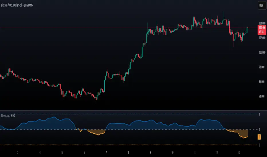
The Hurst Exponent Oscillator (HEO) by PhenLabs is a powerful tool developed for traders who want to distinguish between trending, mean-reverting, and random market behaviors with clarity and precision. By estimating the Hurst Exponent—a statistical measure of long-term memory in financial time series—this indicator helps users make sense of underlying market dynamics that are often not visible through traditional moving averages or oscillators.
Traders can quickly know if the market is likely to continue its current direction (trending), revert to the mean, or behave randomly, allowing for more strategic timing of entries and exits. With customizable smoothing and clear visual cues, the HEO enhances decision-making in a wide range of trading environments.
🚀 Points of Innovation
Integrates advanced Hurst Exponent calculation via Rescaled Range (R/S) analysis, providing unique market character insights.
Offers real-time visual cues for trending, mean-reverting, or random price action zones.
User-controllable EMA smoothing reduces noise for clearer interpretation.
Dynamic coloring and fill for immediate visual categorization of market regime.
Configurable visual thresholds for critical Hurst levels (e.g., 0.4, 0.5, 0.6).
Fully customizable appearance settings to fit different charting preferences.
🔧 Core Components
Log Returns Calculation: Computes log returns of the selected price source to feed into the Hurst calculation, ensuring robust and scale-independent analysis.
Rescaled Range (R/S) Analysis: Assesses the dispersion and cumulative deviation over a rolling window, forming the core statistical basis for the Hurst exponent estimate.
Smoothing Engine: Applies Exponential Moving Average (EMA) smoothing to the raw Hurst value for enhanced clarity.
Dynamic Rolling Windows: Utilizes arrays to maintain efficient, real-time calculations over user-defined lengths.
Adaptive Color Logic: Assigns different highlight and fill colors based on the current Hurst value zone.
🔥 Key Features
Visually differentiates between trending, mean-reverting, and random market modes.
User-adjustable lookback and smoothing periods for tailored sensitivity.
Distinct fill and line styles for each regime to avoid ambiguity.
On-chart reference lines for strong trending and mean-reverting thresholds.
Works with any price series (close, open, HL2, etc.) for versatile application.
🎨 Visualization
Hurst Exponent Curve: Primary plotted line (smoothed if EMA is used) reflects the ongoing estimate of the Hurst exponent.
Colored Zone Filling: The area between the Hurst line and the 0.5 reference line is filled, with color and opacity dynamically indicating the current market regime.
Reference Lines: Dash/dot lines mark standard Hurst thresholds (0.4, 0.5, 0.6) to contextualize the current regime.
All visual elements can be customized for thickness, color intensity, and opacity for user preference.
📖 Usage Guidelines
Data Settings
Hurst Calculation Length
Default: 100
Range: 10-300
Description: Number of bars used in Hurst calculation; higher values mean longer-term analysis, lower values for quicker reaction.
Data Source
Default: close
Description: Select which data series to analyze (e.g., Close, Open, HL2).
Smoothing Length (EMA)
Default: 5
Range: 1-50
Description: Length for smoothing the Hurst value; higher settings yield smoother but less responsive results.
Style Settings
Trending Color (Hurst > 0.5)
Default: Blue tone
Description: Color used when trending regime is detected.
Mean-Reverting Color (Hurst < 0.5)
Default: Orange tone
Description: Color used when mean-reverting regime is detected.
Neutral/Random Color
Default: Soft blue
Description: Color when market behavior is indeterminate or shifting.
Fill Opacity
Default: 70-80
Range: 0-100
Description: Transparency of area fills—higher opacity for stronger visual effect.
Line Width
Default: 2
Range: 1-5
Description: Thickness of the main indicator curve.
✅ Best Use Cases
Identifying if a market is regime-shifting from trending to mean-reverting (or vice versa).
Filtering signals in automated or systematic trading strategies.
Spotting periods of randomness where trading signals should be deprioritized.
Enhancing mean-reversion or trend-following models with regime-awareness.
⚠️ Limitations
Not predictive: Reflects current and recent market state, not future direction.
Sensitive to input parameters—overfitting may occur if settings are changed too frequently.
Smoothing can introduce lag in regime recognition.
May not work optimally in markets with structural breaks or extreme volatility.
💡 What Makes This Unique
Employs advanced statistical market analysis (Hurst exponent) rarely found in standard toolkits.
Offers immediate regime visualization through smart dynamic coloring and zone fills.
🔬 How It Works
Rolling Log Return Calculation:
Each new price creates a log return, forming the basis for robust, non-linear analysis. This ensures all price differences are treated proportionally.
Rescaled Range Analysis:
A rolling window maintains cumulative deviations and computes the statistical “range” (max-min of deviations). This is compared against the standard deviation to estimate “memory”.
Exponent Calculation & Smoothing:
The raw Hurst value is translated from the log of the rescaled range ratio, and then optionally smoothed via EMA to dampen noise and false signals.
Regime Detection Logic:
The smoothed value is checked against 0.5. Values above = trending; below = mean-reverting; near 0.5 = random. These control plot/fill color and zone display.
💡 Note:
Use longer calculation lengths for major market character study, and shorter ones for tactical, short-term adaptation. Smoothing balances noise vs. lag—find a best fit for your trading style. Always combine regime awareness with broader technical/fundamental context for best results.
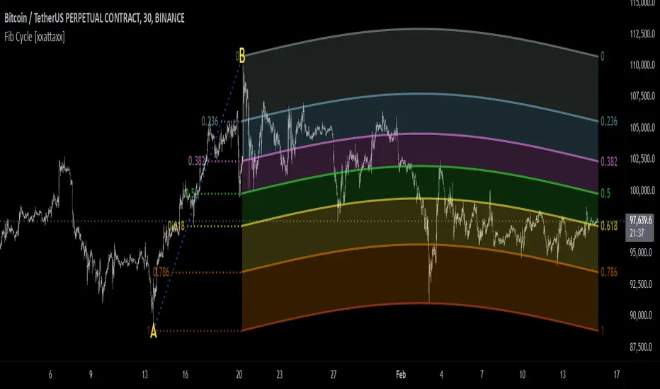
Fibonacci Cycle Finder🟩 Fibonacci Cycle Finder is an indicator designed to explore Fibonacci-based waves and cycles through visualization and experimentation, introducing a trigonometric approach to market structure analysis. Unlike traditional Fibonacci tools that rely on static horizontal levels, this indicator incorporates the dynamic nature of market cycles, using adjustable wavelength, phase, and amplitude settings to visualize the rhythm of price movements. By applying a sine function, it provides a structured way to examine Fibonacci relationships in a non-linear context.
Fibonacci Cycle Finder unifies Fibonacci principles with a wave-based method by employing adjustable parameters to align each wave with real-time price action. By default, the wave begins with minimal curvature, preserving the structural familiarity of horizontal Fibonacci retracements. By adjusting the input parameters, the wave can subtly transition from a horizontal line to a more pronounced cycle,visualizing cyclical structures within price movement. This projective structure extends potential cyclical outlines on the chart, opening deeper exploration of how Fibonacci relationships may emerge over time.
Fibonacci Cycle Finder further underscores a non-linear representation of price by illustrating how wave-based logic can uncover shifts that are missed by static retracement tools. Rather than imposing immediate oscillatory behavior, the indicator encourages a progressive approach, where the parameters may be incrementally modified to align wave structures with observed price action. This refinement process deepens the exploration of Fibonacci relationships, offering a systematic way to experiment with non-linear price dynamics. In doing so, it revisits fundamental Fibonacci concepts, demonstrating their broader adaptability beyond fixed horizontal retracements.
🌀 THEORY & CONCEPT 🌀
What if Fibonacci relationships could be visualized as dynamic waves rather than confined to fixed horizontal levels? Fibonacci Cycle Finder introduces a trigonometric approach to market structure analysis, offering a different perspective on Fibonacci-based cycles. This tool provides a way to visualize market fluctuations through cyclical wave motion, opening the door to further exploration of Fibonacci’s role in non-linear price behavior.
Traditional Fibonacci tools, such as retracements and extensions, have long been used to identify potential support and resistance levels. While valuable for analyzing price trends, these tools assume linear price movement and rely on static horizontal levels. However, market fluctuations often exhibit cyclical tendencies , where price follows natural wave-like structures rather than strictly adhering to fixed retracement points. Although Fibonacci-based tools such as arcs, fans, and time zones attempt to address these patterns, they primarily apply geometric projections. The Fibonacci Cycle Finder takes a different approach by mapping Fibonacci ratios along structured wave cycles, aligning these relationships with the natural curvature of market movement rather than forcing them onto rigid price levels.
Rather than replacing traditional Fibonacci methods, the Fibonacci Cycle Finder supplements existing Fibonacci theory by introducing an exploratory approach to price structure analysis. It encourages traders to experiment with how Fibonacci ratios interact with cyclical price structures, offering an additional layer of insight beyond static retracements and extensions. This approach allows Fibonacci levels to be examined beyond their traditional static form, providing deeper insights into market fluctuations.
📊 FIBONACCI WAVE IMPLEMENTATION 📊
The Fibonacci Cycle Finder uses two user-defined swing points, A and B, as the foundation for projecting these Fibonacci waves. It first establishes standard horizontal levels that correspond to traditional Fibonacci retracements, ensuring a baseline reference before wave adjustments are applied. By default, the wave is intentionally subtle— Wavelength is set to 1 , Amplitude is set to 1 , and Phase is set to 0 . In other words, the wave starts as “stretched out.” This allows a slow, measured start, encouraging users to refine parameters incrementally rather than producing abrupt oscillations. As these parameters are increased, the wave takes on more distinct sine and cosine characteristics, offering a flexible approach to exploring Fibonacci-based cyclicity within price action.
Three parameters control the shape of the Fibonacci wave:
1️⃣ Wavelength Controls the horizontal spacing of the wave along the time axis, determining the length of one full cycle from peak to peak (or trough to trough). In this indicator, Wavelength acts as a scaling input that adjusts how far the wave extends across time, rather than a strict mathematical “wavelength.” Lower values further stretch the wave, increasing the spacing between oscillations, while higher values compress it into a more frequent cycle. Each full cycle is divided into four quarter-cycle segments, a deliberate design choice to minimize curvature by default. This allows for subtle oscillations and smoother transitions, preventing excessive distortion while maintaining flexibility in wave projections. The wavelength is calculated relative to the A-B swing, ensuring that its scale adapts dynamically to the selected price range.
2️⃣ Amplitude Defines the vertical displacement of the wave relative to the baseline Fibonacci level. Higher values increase the height of oscillations, while lower values reduce the height, Negative values will invert the wave’s initial direction. The amplitude is dynamically applied in relation to the A-B swing direction, ensuring that an upward swing results in upward oscillations and a downward swing results in downward oscillations.
3️⃣ Phase Shifts the wave’s starting position along its cycle, adjusting alignment relative to the swing points. A phase of 0 aligns with a sine wave, where the cycle starts at zero and rises. A phase of 25 aligns with a cosine wave, starting at a peak and descending. A phase of 50 inverts the sine wave, beginning at zero but falling first, while a phase of 75 aligns with an inverted cosine , starting at a trough and rising. Intermediate values between these phases create gradual shifts in wave positioning, allowing for finer alignment with observed market structures.
By fine-tuning these parameters, users can adapt Fibonacci waves to better reflect observed market behaviors. The wave structure integrates with price movements rather than simply overlaying static levels, allowing for a more dynamic representation of cyclical price tendencies. This indicator serves as an exploratory tool for understanding potential market rhythms, encouraging traders to test and visualize how Fibonacci principles extend beyond their traditional applications.
🖼️ CHART EXAMPLES 🖼️
Following this downtrend, price interacts with curved Fibonacci levels, highlighting resistance at the 0.236 and 0.382 levels, where price stalls before pulling back. Support emerges at the 0.5, 0.618, and 0.786 levels, where price finds stability and rebounds
In this Fibonacci retracement, price initially finds support at the 1.0 level, following the natural curvature of the cycle. Resistance forms at 0.786, leading to a pullback before price breaks through and tests 0.618 as resistance. Once 0.618 is breached, price moves upward to test 0.5, illustrating how Fibonacci-based cycles may align with evolving market structure beyond static, horizontal retracements.
Following this uptrend, price retraces downward and interacts with the Fibonacci levels, demonstrating both support and resistance at key levels such as 0.236, 0.382, 0.5, and 0.618.
With only the 0.5 and 1.0 levels enabled, this chart remains uncluttered while still highlighting key price interactions. The short cycle length results in a mild curvature, aligning smoothly with market movement. Price finds resistance at the 0.5 level while showing strong support at 1.0, which follows the natural flow of the market. Keeping the focus on fewer levels helps maintain clarity while still capturing how price reacts within the cycle.
🛠️ CONFIGURATION AND SETTINGS 🛠️
Wave Parameters
Wavelength : Stretches or compresses the wave along the time axis, determining the length of one full cycle. Higher values extend the wave across more bars, while lower values compress it into a shorter time frame.
Amplitude : Expands or contracts the wave along the price axis, determining the height of oscillations relative to Fibonacci levels. Higher values increase the vertical range, while negative values invert the wave’s initial direction.
Phase : Offsets the wave along the time axis, adjusting where the cycle begins. Higher values shift the starting position forward within the wave pattern.
Fibonacci Levels
Levels : Enable or disable specific Fibonacci levels (0.0, 0.236, 0.382, 0.5, 0.618, 0.786, 1.0) to focus on relevant price zones.
Color : Modify level colors for enhanced visual clarity.
Visibility
Trend Line/Color : Toggle and customize the trend line connecting swing points A and B.
Setup Lines : Show or hide lines linking Fibonacci levels to projected waves.
A/B Labels Visibility : Control the visibility of swing point labels.
Left/Right Labels : Manage the display of Fibonacci level labels on both sides of the chart.
Fill % : Adjust shading intensity between Fibonacci levels (0% = no fill, 100% = maximum fill).
A and B Points (Time/Price):
These user-defined anchor points serve as the basis for Fibonacci wave calculations and can be manually set. A and B points can also be adjusted directly on the chart, with automatic synchronization to the settings panel, allowing for seamless modifications without needing to manually input values.
⚠️ DISCLAIMER ⚠️
The Fibonacci Cycle Finder is a visual analysis tool designed to illustrate Fibonacci relationships and serve as a supplement to traditional Fibonacci tools. While the indicator employs mathematical and geometric principles, no guarantee is made that its calculations will align with other Fibonacci tools or proprietary methods. Like all technical and visual indicators, the Fibonacci levels generated by this tool may appear to visually align with key price zones in hindsight. However, these levels are not intended as standalone signals for trading decisions. This indicator is intended for educational and analytical purposes, complementing other tools and methods of market analysis.
🧠 BEYOND THE CODE 🧠
Fibonacci Cycle Finder is the latest indicator in the Fibonacci Geometry Series. Building on the concepts of the Fibonacci Time-Price Zones and the Fibonacci 3-D indicators, this tool introduces a trigonometric approach to market structure analysis.
The Fibonacci Cycle Finder indicator, like other xxattaxx indicators , is designed to encourage both education and community engagement. Your feedback and insights are invaluable to refining and enhancing the Fibonacci Cycle Finder indicator. We look forward to the creative applications, observations, and discussions this tool inspires within the trading community.
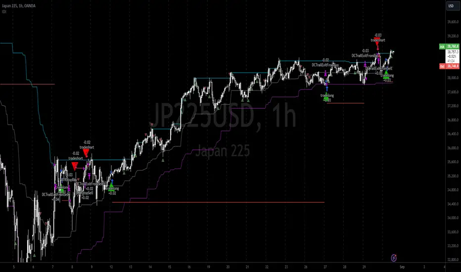
Intramarket Difference Index StrategyHi Traders !!
The IDI Strategy:
In layman’s terms this strategy compares two indicators across markets and exploits their differences.
note: it is best the two markets are correlated as then we know we are trading a short to long term deviation from both markets' general trend with the assumption both markets will trend again sometime in the future thereby exhausting our trading opportunity.
📍 Import Notes:
This Strategy calculates trade position size independently (i.e. risk per trade is controlled in the user inputs tab), this means that the ‘Order size’ input in the ‘Properties’ tab will have no effect on the strategy. Why ? because this allows us to define custom position size algorithms which we can use to improve our risk management and equity growth over time. Here we have the option to have fixed quantity or fixed percentage of equity ATR (Average True Range) based stops in addition to the turtle trading position size algorithm.
‘Pyramiding’ does not work for this strategy’, similar to the order size input togeling this input will have no effect on the strategy as the strategy explicitly defines the maximum order size to be 1.
This strategy is not perfect, and as of writing of this post I have not traded this algo.
Always take your time to backtests and debug the strategy.
🔷 The IDI Strategy:
By default this strategy pulls data from your current TV chart and then compares it to the base market, be default BINANCE:BTCUSD . The strategy pulls SMA and RSI data from either market (we call this the difference data), standardizes the data (solving the different unit problem across markets) such that it is comparable and then differentiates the data, calling the result of this transformation and difference the Intramarket Difference (ID). The formula for the the ID is
ID = market1_diff_data - market2_diff_data (1)
Where
market(i)_diff_data = diff_data / ATR(j)_market(i)^0.5,
where i = {1, 2} and j = the natural numbers excluding 0
Formula (1) interpretation is the following
When ID > 0: this means the current market outperforms the base market
When ID = 0: Markets are at long run equilibrium
When ID < 0: this means the current market underperforms the base market
To form the strategy we define one of two strategy type’s which are Trend and Mean Revesion respectively.
🔸 Trend Case:
Given the ‘‘Strategy Type’’ is equal to TREND we define a threshold for which if the ID crosses over we go long and if the ID crosses under the negative of the threshold we go short.
The motivating idea is that the ID is an indicator of the two symbols being out of sync, and given we know volatility clustering, momentum and mean reversion of anomalies to be a stylised fact of financial data we can construct a trading premise. Let's first talk more about this premise.
For some markets (cryptocurrency markets - synthetic symbols in TV) the stylised fact of momentum is true, this means that higher momentum is followed by higher momentum, and given we know momentum to be a vector quantity (with magnitude and direction) this momentum can be both positive and negative i.e. when the ID crosses above some threshold we make an assumption it will continue in that direction for some time before executing back to its long run equilibrium of 0 which is a reasonable assumption to make if the market are correlated. For example for the BTCUSD - ETHUSD pair, if the ID > +threshold (inputs for MA and RSI based ID thresholds are found under the ‘‘INTRAMARKET DIFFERENCE INDEX’’ group’), ETHUSD outperforms BTCUSD, we assume the momentum to continue so we go long ETHUSD.
In the standard case we would exit the market when the IDI returns to its long run equilibrium of 0 (for the positive case the ID may return to 0 because ETH’s difference data may have decreased or BTC’s difference data may have increased). However in this strategy we will not define this as our exit condition, why ?
This is because we want to ‘‘let our winners run’’, to achieve this we define a trailing Donchian Channel stop loss (along with a fixed ATR based stop as our volatility proxy). If we were too use the 0 exit the strategy may print a buy signal (ID > +threshold in the simple case, market regimes may be used), return to 0 and then print another buy signal, and this process can loop may times, this high trade frequency means we fail capture the entire market move lowering our profit, furthermore on lower time frames this high trade frequencies mean we pay more transaction costs (due to price slippage, commission and big-ask spread) which means less profit.
By capturing the sum of many momentum moves we are essentially following the trend hence the trend following strategy type.
Here we also print the IDI (with default strategy settings with the MA difference type), we can see that by letting our winners run we may catch many valid momentum moves, that results in a larger final pnl that if we would otherwise exit based on the equilibrium condition(Valid trades are denoted by solid green and red arrows respectively and all other valid trades which occur within the original signal are light green and red small arrows).
another example...
Note: if you would like to plot the IDI separately copy and paste the following code in a new Pine Script indicator template.
indicator("IDI")
// INTRAMARKET INDEX
var string g_idi = "intramarket diffirence index"
ui_index_1 = input.symbol("BINANCE:BTCUSD", title = "Base market", group = g_idi)
// ui_index_2 = input.symbol("BINANCE:ETHUSD", title = "Quote Market", group = g_idi)
type = input.string("MA", title = "Differrencing Series", options = , group = g_idi)
ui_ma_lkb = input.int(24, title = "lookback of ma and volatility scaling constant", group = g_idi)
ui_rsi_lkb = input.int(14, title = "Lookback of RSI", group = g_idi)
ui_atr_lkb = input.int(300, title = "ATR lookback - Normalising value", group = g_idi)
ui_ma_threshold = input.float(5, title = "Threshold of Upward/Downward Trend (MA)", group = g_idi)
ui_rsi_threshold = input.float(20, title = "Threshold of Upward/Downward Trend (RSI)", group = g_idi)
//>>+----------------------------------------------------------------+}
// CUSTOM FUNCTIONS |
//<<+----------------------------------------------------------------+{
// construct UDT (User defined type) containing the IDI (Intramarket Difference Index) source values
// UDT will hold many variables / functions grouped under the UDT
type functions
float Close // close price
float ma // ma of symbol
float rsi // rsi of the asset
float atr // atr of the asset
// the security data
getUDTdata(symbol, malookback, rsilookback, atrlookback) =>
indexHighTF = barstate.isrealtime ? 1 : 0
= request.security(symbol, timeframe = timeframe.period,
expression = [close , // Instentiate UDT variables
ta.sma(close, malookback) ,
ta.rsi(close, rsilookback) ,
ta.atr(atrlookback) ])
data = functions.new(close_, ma_, rsi_, atr_)
data
// Intramerket Difference Index
idi(type, symbol1, malookback, rsilookback, atrlookback, mathreshold, rsithreshold) =>
threshold = float(na)
index1 = getUDTdata(symbol1, malookback, rsilookback, atrlookback)
index2 = getUDTdata(syminfo.tickerid, malookback, rsilookback, atrlookback)
// declare difference variables for both base and quote symbols, conditional on which difference type is selected
var diffindex1 = 0.0, var diffindex2 = 0.0,
// declare Intramarket Difference Index based on series type, note
// if > 0, index 2 outpreforms index 1, buy index 2 (momentum based) until equalibrium
// if < 0, index 2 underpreforms index 1, sell index 1 (momentum based) until equalibrium
// for idi to be valid both series must be stationary and normalised so both series hae he same scale
intramarket_difference = 0.0
if type == "MA"
threshold := mathreshold
diffindex1 := (index1.Close - index1.ma) / math.pow(index1.atr*malookback, 0.5)
diffindex2 := (index2.Close - index2.ma) / math.pow(index2.atr*malookback, 0.5)
intramarket_difference := diffindex2 - diffindex1
else if type == "RSI"
threshold := rsilookback
diffindex1 := index1.rsi
diffindex2 := index2.rsi
intramarket_difference := diffindex2 - diffindex1
//>>+----------------------------------------------------------------+}
// STRATEGY FUNCTIONS CALLS |
//<<+----------------------------------------------------------------+{
// plot the intramarket difference
= idi(type,
ui_index_1,
ui_ma_lkb,
ui_rsi_lkb,
ui_atr_lkb,
ui_ma_threshold,
ui_rsi_threshold)
//>>+----------------------------------------------------------------+}
plot(intramarket_difference, color = color.orange)
hline(type == "MA" ? ui_ma_threshold : ui_rsi_threshold, color = color.green)
hline(type == "MA" ? -ui_ma_threshold : -ui_rsi_threshold, color = color.red)
hline(0)
Note it is possible that after printing a buy the strategy then prints many sell signals before returning to a buy, which again has the same implication (less profit. Potentially because we exit early only for price to continue upwards hence missing the larger "trend"). The image below showcases this cenario and again, by allowing our winner to run we may capture more profit (theoretically).
This should be clear...
🔸 Mean Reversion Case:
We stated prior that mean reversion of anomalies is an standerdies fact of financial data, how can we exploit this ?
We exploit this by normalizing the ID by applying the Ehlers fisher transformation. The transformed data is then assumed to be approximately normally distributed. To form the strategy we employ the same logic as for the z score, if the FT normalized ID > 2.5 (< -2.5) we buy (short). Our exit conditions remain unchanged (fixed ATR stop and trailing Donchian Trailing stop)
🔷 Position Sizing:
If ‘‘Fixed Risk From Initial Balance’’ is toggled true this means we risk a fixed percentage of our initial balance, if false we risk a fixed percentage of our equity (current balance).
Note we also employ a volatility adjusted position sizing formula, the turtle training method which is defined as follows.
Turtle position size = (1/ r * ATR * DV) * C
Where,
r = risk factor coefficient (default is 20)
ATR(j) = risk proxy, over j times steps
DV = Dollar Volatility, where DV = (1/Asset Price) * Capital at Risk
🔷 Risk Management:
Correct money management means we can limit risk and increase reward (theoretically). Here we employ
Max loss and gain per day
Max loss per trade
Max number of consecutive losing trades until trade skip
To read more see the tooltips (info circle).
🔷 Take Profit:
By defualt the script uses a Donchain Channel as a trailing stop and take profit, In addition to this the script defines a fixed ATR stop losses (by defualt, this covers cases where the DC range may be to wide making a fixed ATR stop usefull), ATR take profits however are defined but optional.
ATR SL and TP defined for all trades
🔷 Hurst Regime (Regime Filter):
The Hurst Exponent (H) aims to segment the market into three different states, Trending (H > 0.5), Random Geometric Brownian Motion (H = 0.5) and Mean Reverting / Contrarian (H < 0.5). In my interpretation this can be used as a trend filter that eliminates market noise.
We utilize the trending and mean reverting based states, as extra conditions required for valid trades for both strategy types respectively, in the process increasing our trade entry quality.
🔷 Example model Architecture:
Here is an example of one configuration of this strategy, combining all aspects discussed in this post.
Future Updates
- Automation integration (next update)
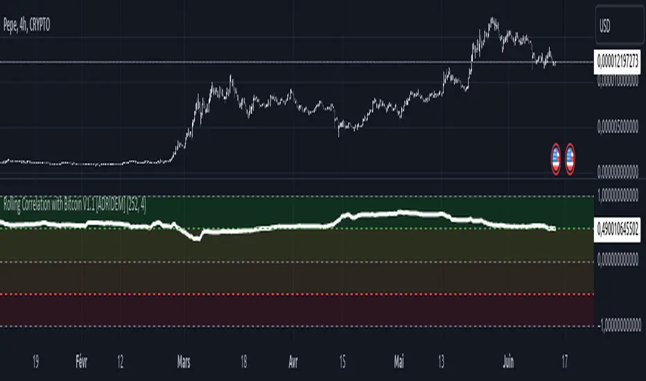
Rolling Correlation with Bitcoin V1.1 [ADRIDEM]Overview
The Rolling Correlation with Bitcoin script is designed to offer a comprehensive view of the correlation between the selected ticker and Bitcoin. This script helps investors understand the relationship between the performance of the current ticker and Bitcoin over a rolling period, providing insights into their interconnected behavior. Below is a detailed presentation of the script and its unique features.
Unique Features of the New Script
Bitcoin Comparison : Allows users to compare the correlation of the current ticker with Bitcoin, providing an analysis of their relationship.
Customizable Rolling Window : Enables users to set the length for the rolling window, adapting to different market conditions and timeframes. The default value is 252 bars, which approximates one year of trading days, but it can be adjusted as needed.
Smoothing Option : Includes an option to apply a smoothing simple moving average (SMA) to the correlation coefficient, helping to reduce noise and highlight trends. The smoothing length is customizable, with a default value of 4 bars.
Visual Indicators : Plots the smoothed correlation coefficient between the current ticker and Bitcoin, with distinct colors for easy interpretation. Additionally, horizontal lines help identify key levels of correlation.
Dynamic Background Color : Adds dynamic background colors to highlight areas of strong positive and negative correlations, enhancing visual clarity.
Originality and Usefulness
This script uniquely combines the analysis of rolling correlation for a current ticker with Bitcoin, providing a comparative view of their relationship. The inclusion of a customizable rolling window and smoothing option enhances its adaptability and usefulness in various market conditions.
Signal Description
The script includes several features that highlight potential insights into the correlation between the assets:
Rolling Correlation with Bitcoin : Plotted as a red line, this represents the smoothed rolling correlation coefficient between the current ticker and Bitcoin.
Horizontal Lines and Background Color : Lines at -0.5, 0, and 0.5 help to quickly identify regions of strong negative, weak, and strong positive correlations.
These features assist in identifying the strength and direction of the relationship between the current ticker and Bitcoin.
Detailed Description
Input Variables
Length for Rolling Window (`length`) : Defines the range for calculating the rolling correlation coefficient. Default is 252.
Smoothing Length (`smoothing_length`) : The number of periods for the smoothing SMA. Default is 4.
Bitcoin Ticker (`bitcoin_ticker`) : The ticker symbol for Bitcoin. Default is "BINANCE:BTCUSDT".
Functionality
Correlation Calculation : The script calculates the daily returns for both Bitcoin and the current ticker and computes their rolling correlation coefficient.
```pine
bitcoin_close = request.security(bitcoin_ticker, timeframe.period, close)
bitcoin_dailyReturn = ta.change(bitcoin_close) / bitcoin_close
current_dailyReturn = ta.change(close) / close
rolling_correlation = ta.correlation(current_dailyReturn, bitcoin_dailyReturn, length)
```
Smoothing : A simple moving average is applied to the rolling correlation coefficient to smooth the data.
```pine
smoothed_correlation = ta.sma(rolling_correlation, smoothing_length)
```
Plotting : The script plots the smoothed rolling correlation coefficient and includes horizontal lines for key levels.
```pine
plot(smoothed_correlation, title="Rolling Correlation with Bitcoin", color=color.rgb(255, 82, 82, 50), linewidth=2)
h_neg1 = hline(-1, "-1 Line", color=color.gray)
h_neg05 = hline(-0.5, "-0.5 Line", color=color.red)
h0 = hline(0, "Zero Line", color=color.gray)
h_pos05 = hline(0.5, "0.5 Line", color=color.green)
h1 = hline(1, "1 Line", color=color.gray)
fill(h_neg1, h_neg05, color=color.rgb(255, 0, 0, 90), title="Strong Negative Correlation Background")
fill(h_neg05, h0, color=color.rgb(255, 165, 0, 90), title="Weak Negative Correlation Background")
fill(h0, h_pos05, color=color.rgb(255, 255, 0, 90), title="Weak Positive Correlation Background")
fill(h_pos05, h1, color=color.rgb(0, 255, 0, 90), title="Strong Positive Correlation Background")
```
How to Use
Configuring Inputs : Adjust the rolling window length and smoothing length as needed. Ensure the Bitcoin ticker is set to the desired asset for comparison.
Interpreting the Indicator : Use the plotted correlation coefficient and horizontal lines to assess the strength and direction of the relationship between the current ticker and Bitcoin.
Signal Confirmation : Look for periods of strong positive or negative correlation to identify potential co-movements or divergences. The background colors help to highlight these key levels.
This script provides a detailed comparative view of the correlation between the current ticker and Bitcoin, aiding in more informed decision-making by highlighting the strength and direction of their relationship.
Color Stochastic IndicatorThis Pine Script™ indicator, "Color Stochastic Indicator," is designed to visualize the stochastic oscillator with color-coded trends and shaded background levels, providing a clearer understanding of market trends and potential trading signals.
Key Features:
Customizable Parameters:
K Period: The period for the %K line in the stochastic calculation (default: 50).
D Period: The period for the %D line, which is the moving average of %K (default: 13).
Slowing: The slowing factor applied to the stochastic calculation (default: 2).
Smoothing: A factor for additional smoothing of the stochastic values (default: 1.0).
Use Crossover: Option to determine trend based on the crossover of %K and %D lines.
Display Levels: Option to show significant stochastic levels on the chart (0.2, 0.5, 0.8).
Price Field: Selection of the price field used in calculations.
Stoch Width: Line width for the %K line.
Signal Width: Line width for the %D line.
Background Colors:
Upper Level Background: Shaded area between 0.5 and 0.8 with a customizable color.
Lower Level Background: Shaded area between 0.2 and 0.5 with a customizable color.
Color-Coded Trends:
Wait (Gray): Neutral state when no clear trend is detected.
Uptrend (Green): Indicates a potential buying signal.
Downtrend (Red): Indicates a potential selling signal.
Signal Line (Blue): Represents the %D line for clearer signal identification.
Alerts:
Customizable alerts trigger when the trend changes, providing timely notifications for potential trade opportunities.
How It Works:
Stochastic Calculation:
The %K line is calculated based on the selected K Period.
The %D line is a simple moving average (SMA) of the %K line over the D Period.
Additional smoothing is applied to both %K and %D lines using the specified Smoothing factor.
Fisher Transform:
The script applies a Fisher transform to the smoothed %K values, enhancing the clarity of trend signals.
Trend Determination:
If Use Crossover is enabled, the trend is determined based on the crossover of smoothed %K and %D lines.
If Use Crossover is disabled, the trend is determined based on whether the smoothed %K value is above or below 0.5.
Background Shading:
Fixed background colors are applied using hline and fill functions, highlighting the specified levels on the chart (0.2, 0.5, 0.8).
Plotting:
The smoothed %K line is plotted with color coding based on its value relative to the %D line and threshold levels.
The %D line is plotted for reference.
How to Use:
Adding the Indicator:
Copy and paste the provided Pine Script™ code into a new indicator script in TradingView.
Save and add the indicator to your desired chart.
Configuring Parameters:
Adjust the input parameters (K Period, D Period, Slowing, etc.) according to your trading strategy and preferences.
Enable or disable the Use Crossover option based on whether you prefer trend determination by crossover or threshold.
Interpreting Signals:
Observe the color-coded %K line to identify potential buy (green) and sell (red) signals.
Use the shaded background areas to quickly assess overbought (0.5 to 0.8) and oversold (0.2 to 0.5) conditions.
Monitor alerts for trend changes to take timely trading actions.
Alerts Setup:
Set up custom alerts based on the provided alert conditions to receive notifications when the trend changes.
Originality:
This script combines the stochastic oscillator with color-coding and background shading for enhanced visualization.
It introduces a unique Fisher transform application to the smoothed %K values.
The crossover and threshold-based trend determination options provide flexibility for different trading strategies.
Customizable alert messages help traders stay informed about trend changes in real time.
By incorporating these features, the "Color Stochastic Indicator" offers a comprehensive tool for traders seeking to leverage stochastic analysis with improved clarity and actionable insights.

Trend Channels [Cryptoverse]This Indicator dynamically generates and displays on the chart Trend Channels with the pivot points it determines in each market and in each time period. The type of price used to determine the pivot points and create the channels is optional (e.g. close or high, low).
It will help you identify your entry points and stop zones and help you take positions, but it does not contain any buy and sell signals or trading strategies. It creates more successful channels on higher timeframes.
Usage Settings:
---------------------------------------------------
General Settings:
Pivot Period: This field determines how many candles before and after a candle will be counted as a peak or bottom in order to determine the peaks and troughs on the chart.
Trend Channels are created by calculating the Pivot points according to the period set here. (Default value: 6)
Top Pivot Source: Determines which value of the related candle the top pivot points will be based on.
Bottom Pivot Source: Determines which value of the related candle the lower pivot points will be based on.
(Default: closing)
Trend Channels Settings:
Show All Trend Lines: Allows you to show or hide trend channels.
Hide Old Trend Lines: If you activate it, it allows you to hide the channels created in the past other than the current trend channels.
Hide 0.5 Lines: Allows you to hide lines at the Fibonacci 0.5 level.
Hide 0.236 Lines: Allows to hide lines at Fibonacci 0.236 level.
Hide 0.786 Lines: Allows to hide lines at Fibonacci 0.786 level.
Helper Line Format: Allows the helper line that converts a trend line into a channel to be drawn based on percentage or price.
*Note:* When using large time intervals by choosing percentages, there may be situations where the helper lines do not provide full parallels.
Up Trend Color: Indicates the outer color of the Up Trend channel.
Down Trend Color: Indicates the outer color of the Descending Trend channel.
0.5 Trend Color: Specifies the color of the fibonacci 0.5 line drawn for all channels.
0.236 Trend Color: Specifies the color of the fibonacci 0.5 line drawn for all channels.
0.786 Trend Color: Sets the color of the fibonacci 0.5 line drawn for all channels.
Trend Channel Width: Determines the thickness of the channel lines.
Trend Channel Style: Determines the style of the channel lines.

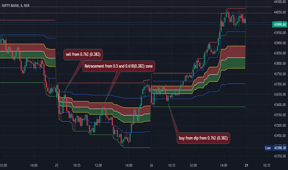
Custom Fib by Dr. MauryaThis indicator is based on purely Fibonacci levels.
How it works:
Let's first understand the Fibonacci levels.
The main Fibonacci numbers are 0, 0.236, 0.392, 0.5, 0.618, 0.764, 1 whereas 0 equal to low and 1 equal to high.
As the market is moving in any direction, new lows or new highs are developing and hence Fibonacci levels are also changing throughout the time.
Sometime market retraces from various levels like 0.5, 0.618/0.382(mirror value), 0.762/0.236 (mirror value).
Retracement : The three mid-level 0.382, 0.5 and 0.618 are act as a retracement or like pivot levels for market. These levels are filled with green and red colors to attention the buyers and sellers to take a trade either side if any candlestick pattern are observed at these levels.
one direction trend takes support of 0.236/0.786(mirror value) (blue line in chart)
Sometime buy/sell on dip levels are happen at 0.762/0.392 (mirror value).
Targets: Target could be Fibonacci extension level lowest targets (1, 1.18, 1.23,), medium targets (1.39, 1.5, 1.61) and large target (2.0, 2.5.2.61, 3.0) as depended on your study volume levels and trend strength.
Stoploss: You can choose any preceding lines for stoploss: e.g. if you enter long on 0.618 or 0.5 levels you can set SL on 0.762
Previous day three mid-point 0.382, 0.5, 0.618 (filled with red and green color) as well as high and low could also act as resistance or support levels for current day market.
Lets understand the Input section of indicator
The first input section allowed to choose where you want to start developing Fibonacci : select session for intraday then weekly, monthly and yearly options are available.
Now you can set any Fibonacci levels (as you wish) you can set upto 20 levels.
By default, total 7 Fibonacci levels are plotted (0, 0.236, 0.392, 0.618, 0.762 and 1.
Further you can set Fibonacci extension level for long side (1.18, 1.23, 1.39, 1.5, 1.61, 2 etc).
You must be careful when you enter Fibonacci extension level lower side (short side). You need to enter value -0.5 (equal to 1.5 for long). -0.618 (equal to 1.618 for long), -1(equal to 2.0 for long).
You can fill color between any two adjacent lines from style sections.
You can also select labels from input tab if you want to see Fibonacci numbers on chart as labels.
You can also shift the labels from current bar to desired offset bar by changing the value in input section.
Conclusion
This indicator is highly customisable developing Fibonacci levels because everyone and different scripts works on different fib levels.
This indicator keeps the Fibonacci levels at a particular time and it plots only new lines when new low or high established without affecting the previous Fibonacci levels. Overall, as the market moves, you will find the trending plot goes which side.
Public Sentiment Oscillator This is a combination of 9 common use indicators turned into on single oscillator. These indicators are: 200 day moving average cross, 9/12 ema cross, 13/48 sma cross, rsi, stochastic, mfi, cci, macd, and open close trend. I have weighted the scores to be pretty even so that its balances each indicator in the sum. Because of the odd number of indicators, I have decided to normalized the score to 10. I think this has the effect of making it easier to read.
The score definition: oc_trend > 0 ? 1 : 0, fast_e > slow_e ? 1 : 0, fast_s > slow_s ? 1 : 0, rsi < 30 ? 0 : rsi > 30 and rsi < 70 ? 0.5 : rsi > 70 ? 1 : 0, macd1 > macd2 ? 0.5 : macd1 < macd2 ? 0 : 0, (hist >=0 ? (hist < hist ? 0.5 : 0.25) : (hist < hist ? 0.25 : 0)), stoch < 20 ? 0 : stoch > 20 and stoch < 80 ? 0.5 : stoch > 80 ? 1 : 0, source > ma200 ? 1 : ex <= ma200 ? 0 : 0, mfi < 20 ? 0 : mfi > 20 and mfi < 80 ? 0.5 : mfi > 80 ? 1 : 0, cci < -100 ? 0 : cci > -100 and cci < 100 ? 0.5 : cci > 100 ? 1 : 0
I hope you find this useful in your trades. Enjoy!

Reset Strike Options-Type 2 (Gray Whaley) [Loxx]For a reset option type 2, the strike is reset in a similar way as a reset option 1. That is, the strike is reset to the asset price at a predetermined future time, if the asset price is below (above) the initial strike price for a call (put). The payoff for such a reset call is max(S - X, 0), and max(X - S, 0) for a put, where X is equal to the original strike X if not reset, and equal to the reset strike if reset. Gray and Whaley (1999) have derived a closed-form solution for the price of European reset strike options. The price of the call option is then given by (via "The Complete Guide to Option Pricing Formulas")
c = Se^(b-r)T2 * M(a1, y1; p) - Xe^(-rT2) * M(a2, y2; p) - Se^(b-r)T1 * N(-a1) * N(z2) * e^-r(T2-T1) + Se^(b-r)T2 * N(-a1) * N(z1)
p = Se^(b-r)T1 * N(a1) * N(-z2) * e^-r(T2-T1) + Se^(b-r)T2 * N(a1) * N(-z1) + Xe^(-rT2) * M(-a2, -y2; p) - Se^(b-r)T2 * M(-a1, -y1; p)
where b is the cost-of-carry of the underlying asset, a is the volatility of the relative price changes in the asset, and r is the risk-free interest rate. K is the strike price of the option, T1 the time to reset (in years), and T2 is its time to expiration. N(x) and M(a,b; p) are, respectively, the univariate and bivariate cumulative normal distribution functions. Further
a1 = (log(S/X) + (b+v^2/2)T1) / v*T1^0.5 ... a2 = a1 - v*T1^0.5
z1 = ((b+v^2/2)(T2-T1)) / v*(T2-T1)^0.5 ... z2 = z1 - v*(T2-T1)^0.5
y1 = (log(S/X) + (b+v^2/2)T1) / v*T1^0.5 ... y2 = a1 - v*T1^0.5
and p = (T1/T2)^0.5. For reset options with multiple reset rights, see Dai, Kwok, and Wu (2003) and Liao and Wang (2003).
Inputs
Asset price ( S )
Strike price ( K )
Reset time ( T1 )
Time to maturity ( T2 )
Risk-free rate ( r )
Cost of carry ( b )
Volatility ( s )
Numerical Greeks or Greeks by Finite Difference
Analytical Greeks are the standard approach to estimating Delta, Gamma etc... That is what we typically use when we can derive from closed form solutions. Normally, these are well-defined and available in text books. Previously, we relied on closed form solutions for the call or put formulae differentiated with respect to the Black Scholes parameters. When Greeks formulae are difficult to develop or tease out, we can alternatively employ numerical Greeks - sometimes referred to finite difference approximations. A key advantage of numerical Greeks relates to their estimation independent of deriving mathematical Greeks. This could be important when we examine American options where there may not technically exist an exact closed form solution that is straightforward to work with. (via VinegarHill FinanceLabs)
Numerical Greeks Outputs
Delta D
Elasticity L
Gamma G
DGammaDvol
GammaP G
Vega
DvegaDvol
VegaP
Theta Q (1 day)
Rho r
Rho futures option r
Phi/Rho2
Carry
DDeltaDvol
Speed
Strike Delta
Strike gamma
Things to know
Only works on the daily timeframe and for the current source price.
You can adjust the text size to fit the screen

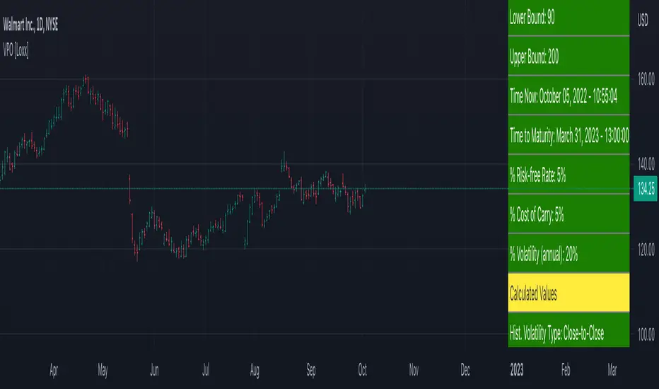
Variable Purchase Options [Loxx]Handley (2001) describes how to value variable purchase options (VPO). A VPO is basically a call option, but where the number of underlying shares is stochastic rather than fixed, or more precisely, a deterministic function of the asset price. The strike price of a VPO is typically a fixed discount to the underlying share price at maturity. The payoff at maturity is equal to max , where N is the number of shares. VPOs may be an interesting tool for firms that need to raise capital relatively far into the future at a given time. The number of underlying shares N is decided on at maturity and is equal to
N = X / St(1 -D)
where X is the strike price, ST is the asset price at maturity, and D is the fixed discount expressed as a proportion 0 > D < 1. The number of shares is in this way a deterministic function of the asset price. Further, the number of shares is often subjected to a minimum and maximum. In this case, we will limit the minimum number of shares to Nmin = X / U(1 -D) if, the asset price at maturity is above a predefined level U at maturity. Similarly, we will reach the maximum number of shares A T = x if the stock price at maturity is equal Nmax = X / L(1 -D) or lower than a predefined level L. Based on Handley (2001), we get the following closed-form solution: (via "The Complete Guide to Option Pricing Formulas")
c = XD / 1-D e^-rT + Nmin(Se^(b-r)T * N(d1) - Ue^-rT * N(d2))
- Nmax(Le^-rT * N(-d4) - Se^(b-r)T * N(-d3))
+ Nmax(L(1-D)e^-rT * N(-d6) - Se^(b-r)T * N(-d5))
where
d1 = (log(S/U) + (b+v^2/2)T) / vT^0.5 ... d2 = d1 - vT^0.5
d3 = (log(S/L) + (b+v^2/2)T) / vT^0.5 ... d4 = d3 - vT^0.5
d5 = (log(S/L(1-D)) + (b+v^2/2)T) / vT^0.5 ... d6 = d5 - vT^0.5
Inputs
Asset price (S)
Strike price (K)
Discount %
Lower bound
Upper bound
Time to maturity
Risk-free rate (r) %
Cost of carry (b) %
Volatility (v) %
Things to know
Only works on the daily timeframe and for the current source price.
You can adjust the text size to fit the screen
American Approximation Bjerksund & Stensland 2002 [Loxx]American Approximation Bjerksund & Stensland 2002 is an American Options pricing model. This indicator also includes numerical greeks. You can compare the output of the American Approximation to the Black-Scholes-Merton value on the output of the options panel.
The Bjerksund & Stensland (2002) Approximation
The Bjerksund and Stensland (2002) approximation divides the time to maturity into two parts, each with a separate flat exercise boundary. It is thus a straightforward generalization of the Bjerksund-Stensland 1993 algorithm. The method is fast and efficient and should be more accurate than the Barone-Adesi and Whaley (1987) and the Bjerksund and Stensland (1993b) approximations. The algorithm requires an accurate cumulative bivariate normal approximation. Several approximations that are described in the literature are not sufficiently accurate, but the Genze algorithm works.
C = alpha2*S^B - alpha2*phi(S, t1, B, I2, I2)
+ phi(S, t1, I2, I2) - phi(S, t1, I, I1, I2)
- X*phi(S, t1, 0, I2, I2) + X*phi(S, t1, 0, I1, I2)
+ alpha1*phi(X, t1, B, I1, I2) - alpha1*psi*St, T, B, I1, I2, I1, t1)
+ psi(S, T, 1, I1, I2, I1, t1) - psi(S, T, 1, X, I2, I1, t1)
- X*psi(S, T, 0, I1, I2, I1, t1) + psi(S, T, 0 ,X, I2, I1, t1)
where
alpha1 = (I1 - X)*I1^-B
alpha2 = (I2 - X)*I2^-B
B = (1/2 - b/v^2) + ((b/v^2 - 1/2)^2 + 2*(r/v^2))^0.5
The function psi(S, T, y, H, I) is given by
psi(S, T, gamma, H, I) = e^lambda * S^gamma * (N(-d) - (I/S)^k * N(-d2))
d = (log(S/H) + (b + (gamma - 1/2) * v^2) * T) / (v * T^0.5)
d2 = (log(I^2/(S*H)) + (b + (gamma - 1/2) * v^2) * T) / (v * T^0.5)
lambda = -r + gamma * b + 1/2 * gamma * (gamma - 1) * v^2
k = 2*b/v^2 + (2 * gamma - 1)
and the trigger price I is defined as
I1 = B0 + (B(+infi) - B0) * (1 - e^h1)
I2 = B0 + (B(+infi) - B0) * (1 - e^h2)
h1 = -(b*t1 + 2*v*t1^0.5) * (X^2 / ((B(+infi) - B0))*B0)
h2 = -(b*T + 2*v*T^0.5) * (X^2 / ((B(+infi) - B0))*B0)
t1 = 1/2 * (5^0.5 - 1) * T
B(+infi) = (B / (B - 1)) * X
B0 = max(X, (r / (r - b)) * X)
Moreover, the function psi(S, T, gamma, H, I2, I1, t1) is given by
psi(S, T, gamma, H, I2, I1, t1, r, b, v) = e^(lambda * T) * S^gamma * (M(-e1, -f1, rho) - (I2/S)^k * M(-e2, -f2, rho)
- (I1/S)^k * M(-e3, -f3, -rho) + (I1/I2)^k * M(-e4, -f4, -rho))
where (see screenshot for e and f values)
b=r options on non-dividend paying stock
b=r-q options on stock or index paying a dividend yield of q
b=0 options on futures
b=r-rf currency options (where rf is the rate in the second currency)
Inputs
S = Stock price.
K = Strike price of option.
T = Time to expiration in years.
r = Risk-free rate
c = Cost of Carry
V = Variance of the underlying asset price
cnd1(x) = Cumulative Normal Distribution
cbnd3(x) = Cumulative Bivariate Normal Distribution
nd(x) = Standard Normal Density Function
convertingToCCRate(r, cmp ) = Rate compounder
Numerical Greeks or Greeks by Finite Difference
Analytical Greeks are the standard approach to estimating Delta, Gamma etc... That is what we typically use when we can derive from closed form solutions. Normally, these are well-defined and available in text books. Previously, we relied on closed form solutions for the call or put formulae differentiated with respect to the Black Scholes parameters. When Greeks formulae are difficult to develop or tease out, we can alternatively employ numerical Greeks - sometimes referred to finite difference approximations. A key advantage of numerical Greeks relates to their estimation independent of deriving mathematical Greeks. This could be important when we examine American options where there may not technically exist an exact closed form solution that is straightforward to work with. (via VinegarHill FinanceLabs)
Things to know
Only works on the daily timeframe and for the current source price.
You can adjust the text size to fit the screen

Modified Bachelier Option Pricing Model w/ Num. Greeks [Loxx]Modified Bachelier Option Pricing Model w/ Num. Greeks is an adaptation of the Modified Bachelier Option Pricing Model in Pine Script. The following information is an except from Espen Gaarder Haug's book "Option Pricing Formulas".
Before Black Scholes Merton
The curious reader may be asking how people priced options before the BSM breakthrough was published in 1973. This section offers a quick overview of some of the most important precursors to the BSM model. As early as 1900, Louis Bachelier published his now famous work on option pricing. In contrast to Black, Scholes, and Merton, Bachelier assumed a normal distribution for the asset price—in other words, an arithmetic Brownian motion process:
dS = sigma * dz
Where S is the asset price and dz is a Wiener process. This implies a positive probability for observing a negative asset price—a feature that is not popular for stocks and any other asset with limited liability features.
The current call price is the expected price at expiration. This argument yields:
c = (S - X)*N(d1) + v * T^0.5 * n(d1)
and for a put option we get
p = (S - X)*N(-d1) + v * T^0.5 * n(d1)
where
d1 = (S - X) / (v * T^0.5)
Modified Bachelier Model
By using the arguments of BSM but now with arithmetic Brownian motion (normal distributed stock price), we can easily correct the Bachelier model to take into account the time value of money in a risk-neutral world. This yields:
c = S * N(d1) - Xe^-rT * N(d1) + v * T^0.5 * n(d1)
p = Xe^-rT * N(-d1) - S * N(-d1) + v * T^0.5 * n(d1)
d1 = (S - X) / (v * T^0.5)
Inputs
S = Stock price.
X = Strike price of option.
T = Time to expiration in years.
r = Risk-free rate
v = Volatility of the underlying asset price
cnd (x) = The cumulative normal distribution function
nd(x) = The standard normal density function
Numerical Greeks or Greeks by Finite Difference
Analytical Greeks are the standard approach to estimating Delta, Gamma etc... That is what we typically use when we can derive from closed form solutions. Normally, these are well-defined and available in text books. Previously, we relied on closed form solutions for the call or put formulae differentiated with respect to the Black Scholes parameters. When Greeks formulae are difficult to develop or tease out, we can alternatively employ numerical Greeks - sometimes referred to finite difference approximations. A key advantage of numerical Greeks relates to their estimation independent of deriving mathematical Greeks. This could be important when we examine American options where there may not technically exist an exact closed form solution that is straightforward to work with. (via VinegarHill FinanceLabs)
Things to know
Volatility for this model is price, so dollars or whatever currency you're using. Historical volatility is also reported in currency.
There is no dividend adjustment input
Only works on the daily timeframe and for the current source price.

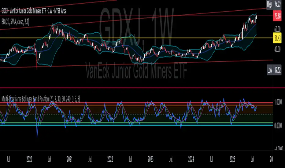
CNS - Multi-Timeframe Bollinger Band OscillatorMy hope is to optimize the settings for this indicator and reintroduce it as a "strategy" with suggested position entry and exit points shown in the price pane.
I’ve been having good results setting the “Bollinger Band MA Length” in the Input tab to between 5 and 10. You can use the standard 20 period, but your results will not be as granular.
This indicator has proven very good at finding local tops and bottoms by combining data from multiple timeframes. Use BB timeframes that are lower than the timeframe you are viewing in your price pane.
The default settings work best on the weekly timeframe, but can be adjusted for most timeframes including intraday.
Be cognizant that the indicator, like other oscillators, does occasionally produce divergences at tops and bottoms.
Any feedback is appreciated.
Overview
This indicator is an oscillator that measures the normalized position of the price relative to Bollinger Bands across multiple timeframes. It takes the price's position within the Bollinger Bands (calculated on different timeframes) and averages those positions to create a single value that oscillates between 0 and 1. This value is then plotted as the oscillator, with reference lines and colored regions to help interpret the price's relative strength or weakness.
How It Works
Bollinger Band Calculation:
The indicator uses a custom function f_getBBPosition() to calculate the position of the price within Bollinger Bands for a given timeframe.
Price Position Normalization:
For each timeframe, the function normalizes the price's position between the upper and lower Bollinger Bands.
It calculates three positions based on the high, low, and close prices of the requested timeframe:
pos_high = (High - Lower Band) / (Upper Band - Lower Band)
pos_low = (Low - Lower Band) / (Upper Band - Lower Band)
pos_close = (Close - Lower Band) / (Upper Band - Lower Band)
If the upper band is not greater than the lower band or if the data is invalid (e.g., na), it defaults to 0.5 (the midline).
The average of these three positions (avg_pos) represents the normalized position for that timeframe, ranging from 0 (at the lower band) to 1 (at the upper band).
Multi-Timeframe Averaging:
The indicator fetches Bollinger Band data from four customizable timeframes (default: 30min, 60min, 240min, daily) using request.security() with lookahead=barmerge.lookahead_on to get the latest available data.
It calculates the normalized position (pos1, pos2, pos3, pos4) for each timeframe using f_getBBPosition().
These four positions are then averaged to produce the final avg_position:avg_position = (pos1 + pos2 + pos3 + pos4) / 4
This average is the oscillator value, which is plotted and typically oscillates between 0 and 1.
Moving Averages:
Two optional moving averages (MA1 and MA2) of the avg_position can be enabled, calculated using simple moving averages (ta.sma) with customizable lengths (default: 5 and 10).
These can be potentially used for MA crossover strategies.
What Is Being Averaged?
The oscillator (avg_position) is the average of the normalized price positions within the Bollinger Bands across the four selected timeframes. Specifically:It averages the avg_pos values (pos1, pos2, pos3, pos4) calculated for each timeframe.
Each avg_pos is itself an average of the normalized positions of the high, low, and close prices relative to the Bollinger Bands for that timeframe.
This multi-timeframe averaging smooths out short-term fluctuations and provides a broader perspective on the price's position within the volatility bands.
Interpretation
0.0 The price is at or below the lower Bollinger Band across all timeframes (indicating potential oversold conditions).
0.15: A customizable level (green band) which can be used for exiting short positions or entering long positions.
0.5: The midline, where the price is at the average of the Bollinger Bands (neutral zone).
0.85: A customizable level (orange band) which can be used for exiting long positions or entering short positions.
1.0: The price is at or above the upper Bollinger Band across all timeframes (indicating potential overbought conditions).
The colored regions and moving averages (if enabled) help identify trends or crossovers for trading signals.
Example
If the 30min timeframe shows the close at the upper band (position = 1.0), the 60min at the midline (position = 0.5), the 240min at the lower band (position = 0.0), and the daily at the upper band (position = 1.0), the avg_position would be:(1.0 + 0.5 + 0.0 + 1.0) / 4 = 0.625
This value (0.625) would plot in the orange region (between 0.85 and 0.5), suggesting the price is relatively strong but not at an extreme.
Notes
The use of lookahead=barmerge.lookahead_on ensures the indicator uses the latest available data, making it more real-time, though its effectiveness depends on the chart timeframe and TradingView's data feed.
The indicator’s sensitivity can be adjusted by changing bb_length ("Bollinger Band MA Length" in the Input tab), bb_mult ("Bollinger Band Standard Deviation," also in the Input tab), or the selected timeframes.

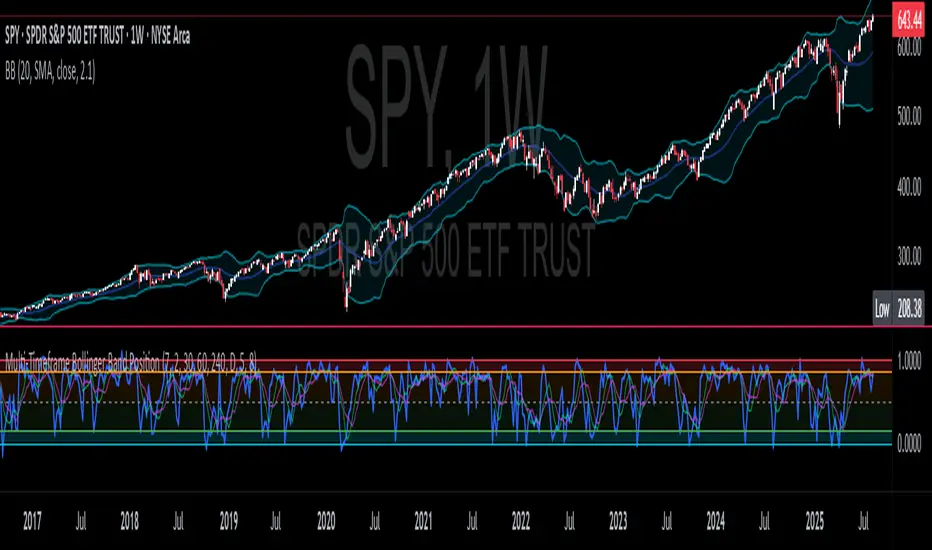
Multi-Timeframe Bollinger BandsMy hope is to optimize the settings for this indicator and reintroduce it as a "strategy" with suggested position entry and exit points shown in the price pane.
I’ve been having good results setting the “Bollinger Band MA Length” in the Input tab to between 5 and 10. You can use the standard 20 period, but your results will not be as granular.
This indicator has proven very good at finding local tops and bottoms by combining data from multiple timeframes. Use timeframes that are lower than the timeframe you are viewing in your price pane. Be cognizant that the indicator, like other oscillators, does occasionally produce divergences at tops and bottoms.
Any feedback is appreciated.
Overview
This indicator is an oscillator that measures the normalized position of the price relative to Bollinger Bands across multiple timeframes. It takes the price's position within the Bollinger Bands (calculated on different timeframes) and averages those positions to create a single value that oscillates between 0 and 1. This value is then plotted as the oscillator, with reference lines and colored regions to help interpret the price's relative strength or weakness.
How It Works
Bollinger Band Calculation:
The indicator uses a custom function f_getBBPosition() to calculate the position of the price within Bollinger Bands for a given timeframe.
Price Position Normalization:
For each timeframe, the function normalizes the price's position between the upper and lower Bollinger Bands.
It calculates three positions based on the high, low, and close prices of the requested timeframe:
pos_high = (High - Lower Band) / (Upper Band - Lower Band)
pos_low = (Low - Lower Band) / (Upper Band - Lower Band)
pos_close = (Close - Lower Band) / (Upper Band - Lower Band)
If the upper band is not greater than the lower band or if the data is invalid (e.g., na), it defaults to 0.5 (the midline).
The average of these three positions (avg_pos) represents the normalized position for that timeframe, ranging from 0 (at the lower band) to 1 (at the upper band).
Multi-Timeframe Averaging:
The indicator fetches Bollinger Band data from four customizable timeframes (default: 30min, 60min, 240min, daily) using request.security() with lookahead=barmerge.lookahead_on to get the latest available data.
It calculates the normalized position (pos1, pos2, pos3, pos4) for each timeframe using f_getBBPosition().
These four positions are then averaged to produce the final avg_position:avg_position = (pos1 + pos2 + pos3 + pos4) / 4
This average is the oscillator value, which is plotted and typically oscillates between 0 and 1.
Moving Averages:
Two optional moving averages (MA1 and MA2) of the avg_position can be enabled, calculated using simple moving averages (ta.sma) with customizable lengths (default: 5 and 10).
These can be potentially used for MA crossover strategies.
What Is Being Averaged?
The oscillator (avg_position) is the average of the normalized price positions within the Bollinger Bands across the four selected timeframes. Specifically:It averages the avg_pos values (pos1, pos2, pos3, pos4) calculated for each timeframe.
Each avg_pos is itself an average of the normalized positions of the high, low, and close prices relative to the Bollinger Bands for that timeframe.
This multi-timeframe averaging smooths out short-term fluctuations and provides a broader perspective on the price's position within the volatility bands.
Interpretation
0.0 The price is at or below the lower Bollinger Band across all timeframes (indicating potential oversold conditions).
0.15: A customizable level (green band) which can be used for exiting short positions or entering long positions.
0.5: The midline, where the price is at the average of the Bollinger Bands (neutral zone).
0.85: A customizable level (orange band) which can be used for exiting long positions or entering short positions.
1.0: The price is at or above the upper Bollinger Band across all timeframes (indicating potential overbought conditions).
The colored regions and moving averages (if enabled) help identify trends or crossovers for trading signals.
Example
If the 30min timeframe shows the close at the upper band (position = 1.0), the 60min at the midline (position = 0.5), the 240min at the lower band (position = 0.0), and the daily at the upper band (position = 1.0), the avg_position would be:(1.0 + 0.5 + 0.0 + 1.0) / 4 = 0.625
This value (0.625) would plot in the orange region (between 0.85 and 0.5), suggesting the price is relatively strong but not at an extreme.
Notes
The use of lookahead=barmerge.lookahead_on ensures the indicator uses the latest available data, making it more real-time, though its effectiveness depends on the chart timeframe and TradingView's data feed.
The indicator’s sensitivity can be adjusted by changing bb_length ("Bollinger Band MA Length" in the Input tab), bb_mult ("Bollinger Band Standard Deviation," also in the Input tab), or the selected timeframes.
Multi-Timeframe Bollinger Band PositionBeta version.
My hope is to optimize the settings for this indicator and reintroduce it as a "strategy" with suggested position entry and exit points shown in the price pane.
Any feedback is appreciated.
Overview
This indicator is an oscillator that measures the normalized position of the price relative to Bollinger Bands across multiple timeframes. It takes the price's position within the Bollinger Bands (calculated on different timeframes) and averages those positions to create a single value that oscillates between 0 and 1. This value is then plotted as the oscillator, with reference lines and colored regions to help interpret the price's relative strength or weakness.
How It Works
Bollinger Band Calculation:
The indicator uses a custom function f_getBBPosition() to calculate the position of the price within Bollinger Bands for a given timeframe.
Price Position Normalization:
For each timeframe, the function normalizes the price's position between the upper and lower Bollinger Bands.
It calculates three positions based on the high, low, and close prices of the requested timeframe:
pos_high = (High - Lower Band) / (Upper Band - Lower Band)
pos_low = (Low - Lower Band) / (Upper Band - Lower Band)
pos_close = (Close - Lower Band) / (Upper Band - Lower Band)
If the upper band is not greater than the lower band or if the data is invalid (e.g., na), it defaults to 0.5 (the midline).
The average of these three positions (avg_pos) represents the normalized position for that timeframe, ranging from 0 (at the lower band) to 1 (at the upper band).
Multi-Timeframe Averaging:
The indicator fetches Bollinger Band data from four customizable timeframes (default: 30min, 60min, 240min, daily) using request.security() with lookahead=barmerge.lookahead_on to get the latest available data.
It calculates the normalized position (pos1, pos2, pos3, pos4) for each timeframe using f_getBBPosition().
These four positions are then averaged to produce the final avg_position:avg_position = (pos1 + pos2 + pos3 + pos4) / 4
This average is the oscillator value, which is plotted and typically oscillates between 0 and 1.
Moving Averages:
Two optional moving averages (MA1 and MA2) of the avg_position can be enabled, calculated using simple moving averages (ta.sma) with customizable lengths (default: 5 and 10).
These can be potentially used for MA crossover strategies.
What Is Being Averaged?
The oscillator (avg_position) is the average of the normalized price positions within the Bollinger Bands across the four selected timeframes. Specifically:It averages the avg_pos values (pos1, pos2, pos3, pos4) calculated for each timeframe.
Each avg_pos is itself an average of the normalized positions of the high, low, and close prices relative to the Bollinger Bands for that timeframe.
This multi-timeframe averaging smooths out short-term fluctuations and provides a broader perspective on the price's position within the volatility bands.
Interpretation:
0.0 The price is at or below the lower Bollinger Band across all timeframes (indicating potential oversold conditions).
0.15: A customizable level (green band) which can be used for exiting short positions or entering long positions.
0.5: The midline, where the price is at the average of the Bollinger Bands (neutral zone).
0.85: A customizable level (orange band) which can be used for exiting long positions or entering short positions.
1.0: The price is at or above the upper Bollinger Band across all timeframes (indicating potential overbought conditions).
The colored regions and moving averages (if enabled) help identify trends or crossovers for trading signals.
Example:
If the 30min timeframe shows the close at the upper band (position = 1.0), the 60min at the midline (position = 0.5), the 240min at the lower band (position = 0.0), and the daily at the upper band (position = 1.0), the avg_position would be:(1.0 + 0.5 + 0.0 + 1.0) / 4 = 0.625
This value (0.625) would plot in the orange region (between 0.85 and 0.5), suggesting the price is relatively strong but not at an extreme.
Notes:
The use of lookahead=barmerge.lookahead_on ensures the indicator uses the latest available data, making it more real-time, though its effectiveness depends on the chart timeframe and TradingView's data feed.
The indicator’s sensitivity can be adjusted by changing bb_length ("Bollinger Band MA Length" in the Input tab), bb_mult ("Bollinger Band Standard Deviation," also in the Input tab), or the selected timeframes.
Active PMI Support/Resistance Levels [EdgeTerminal]The PMI Support & Resistance indicator revolutionizes traditional technical analysis by using Pointwise Mutual Information (PMI) - a statistical measure from information theory - to objectively identify support and resistance levels. Unlike conventional methods that rely on visual pattern recognition, this indicator provides mathematically rigorous, quantifiable evidence of price levels where significant market activity occurs.
- The Mathematical Foundation: Pointwise Mutual Information
Pointwise Mutual Information measures how much more likely two events are to occur together compared to if they were statistically independent. In our context:
Event A: Volume spikes occurring (high trading activity)
Event B: Price being at specific levels
The PMI formula calculates: PMI = log(P(A,B) / (P(A) × P(B)))
Where:
P(A,B) = Probability of volume spikes occurring at specific price levels
P(A) = Probability of volume spikes occurring anywhere
P(B) = Probability of price being at specific levels
High PMI scores indicate that volume spikes and certain price levels co-occur much more frequently than random chance would predict, revealing genuine support and resistance zones.
- Why PMI Outperforms Traditional Methods
Subjective interpretation: What one trader sees as significant, another might ignore
Confirmation bias: Tendency to see patterns that confirm existing beliefs
Inconsistent criteria: No standardized definition of "significant" volume or price action
Static analysis: Doesn't adapt to changing market conditions
No strength measurement: Can't quantify how "strong" a level truly is
PMI Advantages:
✅ Objective & Quantifiable: Mathematical proof of significance, not visual guesswork
✅ Statistical Rigor: Levels backed by information theory and probability
✅ Strength Scoring: PMI scores rank levels by statistical significance
✅ Adaptive: Automatically adjusts to different market volatility regimes
✅ Eliminates Bias: Computer-calculated, removing human interpretation errors
✅ Market Structure Aware: Reveals the underlying order flow concentrations
- How It Works
Data Processing Pipeline:
Volume Analysis: Identifies volume spikes using configurable thresholds
Price Binning: Divides price range into discrete levels for analysis
Co-occurrence Calculation: Measures how often volume spikes happen at each price level
PMI Computation: Calculates statistical significance for each price level
Level Filtering: Shows only levels exceeding minimum PMI thresholds
Dynamic Updates: Refreshes levels periodically while maintaining historical traces
Visual System:
Current Levels: Bright, thick lines with PMI scores - your actionable levels
Historical Traces: Faded previous levels showing market structure evolution
Strength Tiers: Line styles indicate PMI strength (solid/dashed/dotted)
Color Coding: Green for support, red for resistance
Info Table: Real-time display of strongest levels with scores
- Indicator Settings:
Core Parameters
Lookback Period (Default: 200)
Lower (50-100): More responsive to recent price action, catches short-term levels
Higher (300-500): Focuses on major historical levels, more stable but less responsive
Best for: Day trading (100-150), Swing trading (200-300), Position trading (400-500)
Volume Spike Threshold (Default: 1.5)
Lower (1.2-1.4): More sensitive, catches smaller volume increases, more levels detected
Higher (2.0-3.0): Only major volume surges count, fewer but stronger signals
Market dependent: High-volume stocks may need higher thresholds (2.0+), low-volume stocks lower (1.2-1.3)
Price Bins (Default: 50)
Lower (20-30): Broader price zones, less precise but captures wider areas
Higher (70-100): More granular levels, precise but may be overly specific
Volatility dependent: High volatility assets benefit from more bins (70+)
Minimum PMI Score (Default: 0.5)
Lower (0.2-0.4): Shows more levels including weaker ones, comprehensive view
Higher (1.0-2.0): Only statistically strong levels, cleaner chart
Progressive filtering: Start with 0.5, increase if too cluttered
Max Levels to Show (Default: 8)
Fewer (3-5): Clean chart focusing on strongest levels only
More (10-15): Comprehensive view but may clutter chart
Strategy dependent: Scalpers prefer fewer (3-5), swing traders more (8-12)
Historical Tracking Settings
Update Frequency (Default: 20 bars)
Lower (5-10): More frequent updates, captures rapid market changes
Higher (50-100): Less frequent updates, focuses on major structural shifts
Timeframe scaling: 1-minute charts need lower frequency (5-10), daily charts higher (50+)
Show Historical Levels (Default: True)
Enables the "breadcrumb trail" effect showing evolution of support/resistance
Disable for cleaner charts focusing only on current levels
Max Historical Marks (Default: 50)
Lower (20-30): Less memory usage, shorter history
Higher (100-200): Longer historical context but more resource intensive
Fade Strength (Default: 0.8)
Lower (0.5-0.6): Historical levels more visible
Higher (0.9-0.95): Historical levels very subtle
Visual Settings
Support/Resistance Colors: Choose colors that contrast well with your chart theme Line Width: Thicker lines (3-4) for better visibility on busy charts Show PMI Scores: Toggle labels showing statistical strength Label Size: Adjust based on screen resolution and chart zoom level
- Most Effective Usage Strategies
For Day Trading:
Setup: Lookback 100-150, Volume Threshold 1.8-2.2, Update Frequency 10-15
Use PMI levels as bounce/rejection points for scalp entries
Higher PMI scores (>1.5) offer better probability setups
Watch for volume spike confirmations at levels
For Swing Trading:
Setup: Lookback 200-300, Volume Threshold 1.5-2.0, Update Frequency 20-30
Enter on pullbacks to high PMI support levels
Target next resistance level with PMI score >1.0
Hold through minor levels, exit at major PMI levels
For Position Trading:
Setup: Lookback 400-500, Volume Threshold 2.0+, Update Frequency 50+
Focus on PMI scores >2.0 for major structural levels
Use for portfolio entry/exit decisions
Combine with fundamental analysis for timing
- Trading Applications:
Entry Strategies:
PMI Bounce Trades
Price approaches high PMI support level (>1.0)
Wait for volume spike confirmation (orange triangles)
Enter long on bullish price action at the level
Stop loss just below the PMI level
Target: Next PMI resistance level
PMI Breakout Trades
Price consolidates near high PMI level
Volume increases (watch for orange triangles)
Enter on decisive break with volume
Previous resistance becomes new support
Target: Next major PMI level
PMI Rejection Trades
Price approaches PMI resistance with momentum
Watch for rejection signals and volume spikes
Enter short on failure to break through
Stop above the PMI level
Target: Next PMI support level
Risk Management:
Stop Loss Placement
Place stops 0.1-0.5% beyond PMI levels (adjust for volatility)
Higher PMI scores warrant tighter stops
Use ATR-based stops for volatile assets
Position Sizing
Larger positions at PMI levels >2.0 (highest conviction)
Smaller positions at PMI levels 0.5-1.0 (lower conviction)
Scale out at multiple PMI targets
- Key Warning Signs & What to Watch For
Red Flags:
🚨 Very Low PMI Scores (<0.3): Weak statistical significance, avoid trading
🚨 No Volume Confirmation: PMI level without recent volume spikes may be stale
🚨 Overcrowded Levels: Too many levels close together suggests poor parameter tuning
🚨 Outdated Levels: Historical traces are reference only, not tradeable
Optimization Tips:
✅ Regular Recalibration: Adjust parameters monthly based on market regime changes
✅ Volume Context: Always check for recent volume activity at PMI levels
✅ Multiple Timeframes: Confirm PMI levels across different timeframes
✅ Market Conditions: Higher thresholds during high volatility periods
Interpreting PMI Scores
PMI Score Ranges:
0.5-1.0: Moderate statistical significance, proceed with caution
1.0-1.5: Good significance, reliable for most trading strategies
1.5-2.0: Strong significance, high-confidence trade setups
2.0+: Very strong significance, institutional-grade levels
Historical Context: The historical trace system shows how support and resistance evolve over time. When current levels align with multiple historical traces, it indicates persistent market memory at those prices, significantly increasing the level's reliability.
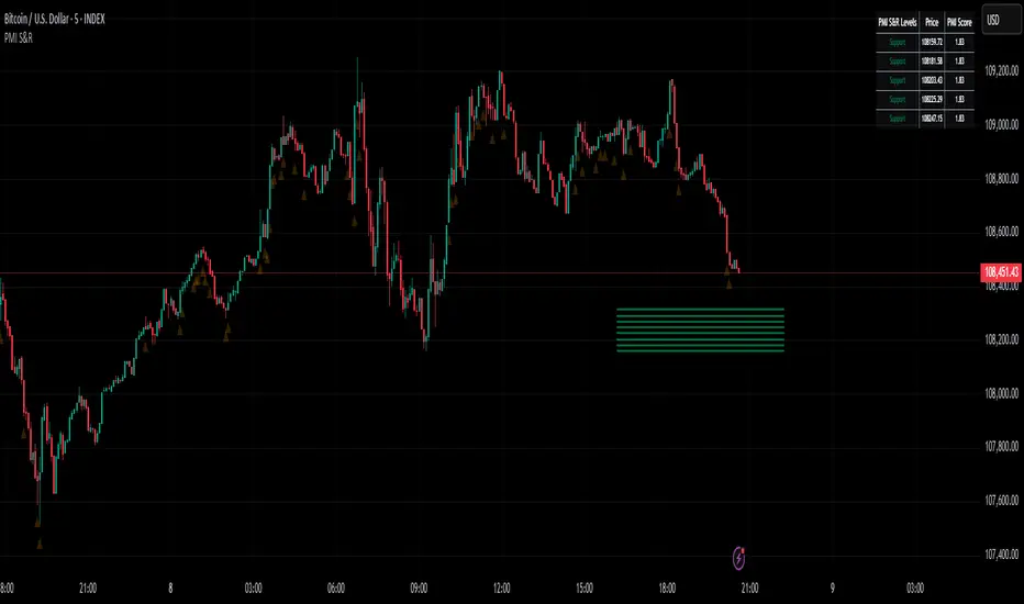
Multifractal Forecast [ScorsoneEnterprises]Multifractal Forecast Indicator
The Multifractal Forecast is an indicator designed to model and forecast asset price movements using a multifractal framework. It uses concepts from fractal geometry and stochastic processes, specifically the Multifractal Model of Asset Returns (MMAR) and fractional Brownian motion (fBm), to generate price forecasts based on historical price data. The indicator visualizes potential future price paths as colored lines, providing traders with a probabilistic view of price trends over a specified trading time scale. Below is a detailed breakdown of the indicator’s functionality, inputs, calculations, and visualization.
Overview
Purpose: The indicator forecasts future price movements by simulating multiple price paths based on a multifractal model, which accounts for the complex, non-linear behavior of financial markets.
Key Concepts:
Multifractal Model of Asset Returns (MMAR): Models price movements as a multifractal process, capturing varying degrees of volatility and self-similarity across different time scales.
Fractional Brownian Motion (fBm): A generalization of Brownian motion that incorporates long-range dependence and self-similarity, controlled by the Hurst exponent.
Binomial Cascade: Used to model trading time, introducing heterogeneity in time scales to reflect market activity bursts.
Hurst Exponent: Measures the degree of long-term memory in the price series (persistence, randomness, or mean-reversion).
Rescaled Range (R/S) Analysis: Estimates the Hurst exponent to quantify the fractal nature of the price series.
Inputs
The indicator allows users to customize its behavior through several input parameters, each influencing the multifractal model and forecast generation:
Maximum Lag (max_lag):
Type: Integer
Default: 50
Minimum: 5
Purpose: Determines the maximum lag used in the rescaled range (R/S) analysis to calculate the Hurst exponent. A higher lag increases the sample size for Hurst estimation but may smooth out short-term dynamics.
2 to the n values in the Multifractal Model (n):
Type: Integer
Default: 4
Purpose: Defines the resolution of the multifractal model by setting the size of arrays used in calculations (N = 2^n). For example, n=4 results in N=16 data points. Larger n increases computational complexity and detail but may exceed Pine Script’s array size limits (capped at 100,000).
Multiplier for Binomial Cascade (m):
Type: Float
Default: 0.8
Purpose: Controls the asymmetry in the binomial cascade, which models trading time. The multiplier m (and its complement 2.0 - m) determines how mass is distributed across time scales. Values closer to 1 create more balanced cascades, while values further from 1 introduce more variability.
Length Scale for fBm (L):
Type: Float
Default: 100,000.0
Purpose: Scales the fractional Brownian motion output, affecting the amplitude of simulated price paths. Larger values increase the magnitude of forecasted price movements.
Cumulative Sum (cum):
Type: Integer (0 or 1)
Default: 1
Purpose: Toggles whether the fBm output is cumulatively summed (1=On, 0=Off). When enabled, the fBm series is accumulated to simulate a price path with memory, resembling a random walk with long-range dependence.
Trading Time Scale (T):
Type: Integer
Default: 5
Purpose: Defines the forecast horizon in bars (20 bars into the future). It also scales the binomial cascade’s output to align with the desired trading time frame.
Number of Simulations (num_simulations):
Type: Integer
Default: 5
Minimum: 1
Purpose: Specifies how many forecast paths are simulated and plotted. More simulations provide a broader range of possible price outcomes but increase computational load.
Core Calculations
The indicator combines several mathematical and statistical techniques to generate price forecasts. Below is a step-by-step explanation of its calculations:
Log Returns (lgr):
The indicator calculates log returns as math.log(close / close ) when both the current and previous close prices are positive. This measures the relative price change in a logarithmic scale, which is standard for financial time series analysis to stabilize variance.
Hurst Exponent Estimation (get_hurst_exponent):
Purpose: Estimates the Hurst exponent (H) to quantify the degree of long-term memory in the price series.
Method: Uses rescaled range (R/S) analysis:
For each lag from 2 to max_lag, the function calc_rescaled_range computes the rescaled range:
Calculate the mean of the log returns over the lag period.
Compute the cumulative deviation from the mean.
Find the range (max - min) of the cumulative deviation.
Divide the range by the standard deviation of the log returns to get the rescaled range.
The log of the rescaled range (log(R/S)) is regressed against the log of the lag (log(lag)) using the polyfit_slope function.
The slope of this regression is the Hurst exponent (H).
Interpretation:
H = 0.5: Random walk (no memory, like standard Brownian motion).
H > 0.5: Persistent behavior (trends tend to continue).
H < 0.5: Mean-reverting behavior (price tends to revert to the mean).
Fractional Brownian Motion (get_fbm):
Purpose: Generates a fractional Brownian motion series to model price movements with long-range dependence.
Inputs: n (array size 2^n), H (Hurst exponent), L (length scale), cum (cumulative sum toggle).
Method:
Computes covariance for fBm using the formula: 0.5 * (|i+1|^(2H) - 2 * |i|^(2H) + |i-1|^(2H)).
Uses Hosking’s method (referenced from Columbia University’s implementation) to generate fBm:
Initializes arrays for covariance (cov), intermediate calculations (phi, psi), and output.
Iteratively computes the fBm series by incorporating a random term scaled by the variance (v) and covariance structure.
Applies scaling based on L / N^H to adjust the amplitude.
Optionally applies cumulative summation if cum = 1 to produce a path with memory.
Output: An array of 2^n values representing the fBm series.
Binomial Cascade (get_binomial_cascade):
Purpose: Models trading time (theta) to account for non-uniform market activity (e.g., bursts of volatility).
Inputs: n (array size 2^n), m (multiplier), T (trading time scale).
Method:
Initializes an array of size 2^n with values of 1.0.
Iteratively applies a binomial cascade:
For each block (from 0 to n-1), splits the array into segments.
Randomly assigns a multiplier (m or 2.0 - m) to each segment, redistributing mass.
Normalizes the array by dividing by its sum and scales by T.
Checks for array size limits to prevent Pine Script errors.
Output: An array (theta) representing the trading time, which warps the fBm to reflect market activity.
Interpolation (interpolate_fbm):
Purpose: Maps the fBm series to the trading time scale to produce a forecast.
Method:
Computes the cumulative sum of theta and normalizes it to .
Interpolates the fBm series linearly based on the normalized trading time.
Ensures the output aligns with the trading time scale (T).
Output: An array of interpolated fBm values representing log returns over the forecast horizon.
Price Path Generation:
For each simulation (up to num_simulations):
Generates an fBm series using get_fbm.
Interpolates it with the trading time (theta) using interpolate_fbm.
Converts log returns to price levels:
Starts with the current close price.
For each step i in the forecast horizon (T), computes the price as prev_price * exp(log_return).
Output: An array of price levels for each simulation.
Visualization:
Trigger: Updates every T bars when the bar state is confirmed (barstate.isconfirmed).
Process:
Clears previous lines from line_array.
For each simulation, plots a line from the current bar’s close price to the forecasted price at bar_index + T.
Colors the line using a gradient (color.from_gradient) based on the final forecasted price relative to the minimum and maximum forecasted prices across all simulations (red for lower prices, teal for higher prices).
Output: Multiple colored lines on the chart, each representing a possible price path over the next T bars.
How It Works on the Chart
Initialization: On each bar, the indicator calculates the Hurst exponent (H) using historical log returns and prepares the trading time (theta) using the binomial cascade.
Forecast Generation: Every T bars, it generates num_simulations price paths:
Each path starts at the current close price.
Uses fBm to model log returns, warped by the trading time.
Converts log returns to price levels.
Plotting: Draws lines from the current bar to the forecasted price T bars ahead, with colors indicating relative price levels.
Dynamic Updates: The forecast updates every T bars, replacing old lines with new ones based on the latest price data and calculations.
Key Features
Multifractal Modeling: Captures complex market dynamics by combining fBm (long-range dependence) with a binomial cascade (non-uniform time).
Customizable Parameters: Allows users to adjust the forecast horizon, model resolution, scaling, and number of simulations.
Probabilistic Forecast: Multiple simulations provide a range of possible price outcomes, helping traders assess uncertainty.
Visual Clarity: Gradient-colored lines make it easy to distinguish bullish (teal) and bearish (red) forecasts.
Potential Use Cases
Trend Analysis: Identify potential price trends or reversals based on the direction and spread of forecast lines.
Risk Assessment: Evaluate the range of possible price outcomes to gauge market uncertainty.
Volatility Analysis: The Hurst exponent and binomial cascade provide insights into market persistence and volatility clustering.
Limitations
Computational Intensity: Large values of n or num_simulations may slow down execution or hit Pine Script’s array size limits.
Randomness: The binomial cascade and fBm rely on random terms (math.random), which may lead to variability between runs.
Assumptions: The model assumes log-normal price movements and fractal behavior, which may not always hold in extreme market conditions.
Adjusting Inputs:
Set max_lag based on the desired depth of historical analysis.
Adjust n for model resolution (start with 4–6 to avoid performance issues).
Tune m to control trading time variability (0.5–1.5 is typical).
Set L to scale the forecast amplitude (experiment with values like 10,000–1,000,000).
Choose T based on your trading horizon (20 for short-term, 50 for longer-term for example).
Select num_simulations for the number of forecast paths (5–10 is reasonable for visualization).
Interpret Output:
Teal lines suggest bullish scenarios, red lines suggest bearish scenarios.
A wide spread of lines indicates high uncertainty; convergence suggests a stronger trend.
Monitor Updates: Forecasts update every T bars, so check the chart periodically for new projections.
Chart Examples
This is a daily AMEX:SPY chart with default settings. We see the simulations being done every T bars and they provide a range for us to analyze with a few simulations still in the range.
On this intraday PEPPERSTONE:COCOA chart I modified the Length Scale for fBm, L, parameter to be 1000 from 100000. Adjusting the parameter as you switch between timeframes can give you more contextual simulations.
On BITSTAMP:ETHUSD I modified the L to be 1000000 to have a more contextual set of simulations with crypto's volatile nature.
With L at 100000 we see the range for NASDAQ:TLT is correctly simulated. The recent pop stays within the bounds of the highest simulation. Note this is a cherry picked example to show the power and potential of these simulations.
Technical Notes
Error Handling: The script includes checks for array size limits and division by zero (math.abs(denominator) > 1e-10, v := math.max(v, 1e-10)).
External Reference: The fBm implementation is based on Hosking’s method (www.columbia.edu), ensuring a robust algorithm.
Conclusion
The Multifractal Forecast is a powerful tool for traders seeking to model complex market dynamics using a multifractal framework. By combining fBm, binomial cascades, and Hurst exponent analysis, it generates probabilistic price forecasts that account for long-range dependence and non-uniform market activity. Its customizable inputs and clear visualizations make it suitable for both technical analysis and strategy development, though users should be mindful of its computational demands and parameter sensitivity. For optimal use, experiment with input settings and validate forecasts against other technical indicators or market conditions.
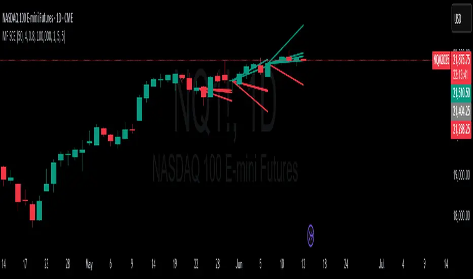
Topological Market Stress (TMS) - Quantum FabricTopological Market Stress (TMS) - Quantum Fabric
What Stresses The Market?
Topological Market Stress (TMS) represents a revolutionary fusion of algebraic topology and quantum field theory applied to financial markets. Unlike traditional indicators that analyze price movements linearly, TMS examines the underlying topological structure of market data—detecting when the very fabric of market relationships begins to tear, warp, or collapse.
Drawing inspiration from the ethereal beauty of quantum field visualizations and the mathematical elegance of topological spaces, this indicator transforms complex mathematical concepts into an intuitive, visually stunning interface that reveals hidden market dynamics invisible to conventional analysis.
Theoretical Foundation: Topology Meets Markets
Topological Holes in Market Structure
In algebraic topology, a "hole" represents a fundamental structural break—a place where the normal connectivity of space fails. In markets, these topological holes manifest as:
Correlation Breakdown: When traditional price-volume relationships collapse
Volatility Clustering Failure: When volatility patterns lose their predictive power
Microstructure Stress: When market efficiency mechanisms begin to fail
The Mathematics of Market Topology
TMS constructs a topological space from market data using three key components:
1. Correlation Topology
ρ(P,V) = correlation(price, volume, period)
Hole Formation = 1 - |ρ(P,V)|
When price and volume decorrelate, topological holes begin forming.
2. Volatility Clustering Topology
σ(t) = volatility at time t
Clustering = correlation(σ(t), σ(t-1), period)
Breakdown = 1 - |Clustering|
Volatility clustering breakdown indicates structural instability.
3. Market Efficiency Topology
Efficiency = |price - EMA(price)| / ATR
Measures how far price deviates from its efficient trajectory.
Multi-Scale Topological Analysis
Markets exist across multiple temporal scales simultaneously. TMS analyzes topology at three distinct scales:
Micro Scale (3-15 periods): Immediate structural changes, market microstructure stress
Meso Scale (10-50 periods): Trend-level topology, medium-term structural shifts
Macro Scale (50-200 periods): Long-term structural topology, regime-level changes
The final stress metric combines all scales:
Combined Stress = 0.3×Micro + 0.4×Meso + 0.3×Macro
How TMS Works
1. Topological Space Construction
Each market moment is embedded in a multi-dimensional topological space where:
- Price efficiency forms one dimension
- Correlation breakdown forms another
- Volatility clustering breakdown forms the third
2. Hole Detection Algorithm
The indicator continuously scans this topological space for:
Hole Formation: When stress exceeds the formation threshold
Hole Persistence: How long structural breaks maintain
Hole Collapse: Sudden topology restoration (regime shifts)
3. Quantum Visualization Engine
The visualization system translates topological mathematics into intuitive quantum field representations:
Stress Waves: Main line showing topological stress intensity
Quantum Glow: Surrounding field indicating stress energy
Fabric Integrity: Background showing structural health
Multi-Scale Rings: Orbital representations of different timeframes
4. Signal Generation
Stable Topology (✨): Normal market structure, standard trading conditions
Stressed Topology (⚡): Increased structural tension, heightened volatility expected
Topological Collapse (🕳️): Major structural break, regime shift in progress
Critical Stress (🌋): Extreme conditions, maximum caution required
Inputs & Parameters
🕳️ Topological Parameters
Analysis Window (20-200, default: 50)
Primary period for topological analysis
20-30: High-frequency scalping, rapid structure detection
50: Balanced approach, recommended for most markets
100-200: Long-term position trading, major structural shifts only
Hole Formation Threshold (0.1-0.9, default: 0.3)
Sensitivity for detecting topological holes
0.1-0.2: Very sensitive, detects minor structural stress
0.3: Balanced, optimal for most market conditions
0.5-0.9: Conservative, only major structural breaks
Density Calculation Radius (0.1-2.0, default: 0.5)
Radius for local density estimation in topological space
0.1-0.3: Fine-grained analysis, sensitive to local changes
0.5: Standard approach, balanced sensitivity
1.0-2.0: Broad analysis, focuses on major structural features
Collapse Detection (0.5-0.95, default: 0.7)
Threshold for detecting sudden topology restoration
0.5-0.6: Very sensitive to regime changes
0.7: Balanced, reliable collapse detection
0.8-0.95: Conservative, only major regime shifts
📊 Multi-Scale Analysis
Enable Multi-Scale (default: true)
- Analyzes topology across multiple timeframes simultaneously
- Provides deeper insight into market structure at different scales
- Essential for understanding cross-timeframe topology interactions
Micro Scale Period (3-15, default: 5)
Fast scale for immediate topology changes
3-5: Ultra-fast, tick/minute data analysis
5-8: Fast, 5m-15m chart optimization
10-15: Medium-fast, 30m-1H chart focus
Meso Scale Period (10-50, default: 20)
Medium scale for trend topology analysis
10-15: Short trend structures
20-25: Medium trend structures (recommended)
30-50: Long trend structures
Macro Scale Period (50-200, default: 100)
Slow scale for structural topology
50-75: Medium-term structural analysis
100: Long-term structure (recommended)
150-200: Very long-term structural patterns
⚙️ Signal Processing
Smoothing Method (SMA/EMA/RMA/WMA, default: EMA) Method for smoothing stress signals
SMA: Simple average, stable but slower
EMA: Exponential, responsive and recommended
RMA: Running average, very smooth
WMA: Weighted average, balanced approach
Smoothing Period (1-10, default: 3)
Period for signal smoothing
1-2: Minimal smoothing, noisy but fast
3-5: Balanced, recommended for most applications
6-10: Heavy smoothing, slow but very stable
Normalization (Fixed/Adaptive/Rolling, default: Adaptive)
Method for normalizing stress values
Fixed: Static 0-1 range normalization
Adaptive: Dynamic range adjustment (recommended)
Rolling: Rolling window normalization
🎨 Quantum Visualization
Fabric Style Options:
Quantum Field: Flowing energy visualization with smooth gradients
Topological Mesh: Mathematical topology with stepped lines
Phase Space: Dynamical systems view with circular markers
Minimal: Clean, simple display with reduced visual elements
Color Scheme Options:
Quantum Gradient: Deep space blue → Quantum red progression
Thermal: Black → Hot orange thermal imaging style
Spectral: Purple → Gold full spectrum colors
Monochrome: Dark gray → Light gray elegant simplicity
Multi-Scale Rings (default: true)
- Display orbital rings for different time scales
- Visualizes how topology changes across timeframes
- Provides immediate visual feedback on cross-scale dynamics
Glow Intensity (0.0-1.0, default: 0.6)
Controls the quantum glow effect intensity
0.0: No glow, pure line display
0.6: Balanced, recommended setting
1.0: Maximum glow, full quantum field effect
📋 Dashboard & Alerts
Show Dashboard (default: true)
Real-time topology status display
Current market state and trading recommendations
Stress level visualization and fabric integrity status
Show Theory Guide (default: true)
Educational panel explaining topological concepts
Dashboard interpretation guide
Trading strategy recommendations
Enable Alerts (default: true)
Extreme stress detection alerts
Topological collapse notifications
Hole formation and recovery signals
Visual Logic & Interpretation
Main Visualization Elements
Quantum Stress Line
Primary indicator showing topological stress intensity
Color intensity reflects current market state
Line style varies based on selected fabric style
Glow effect indicates stress energy field
Equilibrium Line
Silver line showing average stress level
Reference point for normal market conditions
Helps identify when stress is elevated or suppressed
Upper/Lower Bounds
Red upper bound: High stress threshold
Green lower bound: Low stress threshold
Quantum fabric fill between bounds shows stress field
Multi-Scale Rings
Aqua circles : Micro-scale topology (immediate changes)
Orange circles: Meso-scale topology (trend-level changes)
Provides cross-timeframe topology visualization
Dashboard Information
Topology State Icons:
✨ STABLE: Normal market structure, standard trading conditions
⚡ STRESSED: Increased structural tension, monitor closely
🕳️ COLLAPSE: Major structural break, regime shift occurring
🌋 CRITICAL: Extreme conditions, reduce risk exposure
Stress Bar Visualization:
Visual representation of current stress level (0-100%)
Color-coded based on current topology state
Real-time percentage display
Fabric Integrity Dots:
●●●●● Intact: Strong market structure (0-30% stress)
●●●○○ Stressed: Weakening structure (30-70% stress)
●○○○○ Fractured: Breaking down structure (70-100% stress)
Action Recommendations:
✅ TRADE: Normal conditions, standard strategies apply
⚠️ WATCH: Monitor closely, increased vigilance required
🔄 ADAPT: Change strategy, regime shift in progress
🛑 REDUCE: Lower risk exposure, extreme conditions
Trading Strategies
In Stable Topology (✨ STABLE)
- Normal trading conditions apply
- Use standard technical analysis
- Regular position sizing appropriate
- Both trend-following and mean-reversion strategies viable
In Stressed Topology (⚡ STRESSED)
- Increased volatility expected
- Widen stop losses to account for higher volatility
- Reduce position sizes slightly
- Focus on high-probability setups
- Monitor for potential regime change
During Topological Collapse (🕳️ COLLAPSE)
- Major regime shift in progress
- Adapt strategy immediately to new market character
- Consider closing positions that rely on previous regime
- Wait for new topology to stabilize before major trades
- Opportunity for contrarian plays if collapse is extreme
In Critical Stress (🌋 CRITICAL)
- Extreme market conditions
- Significantly reduce risk exposure
- Avoid new positions until stress subsides
- Focus on capital preservation
- Consider hedging existing positions
Advanced Techniques
Multi-Timeframe Topology Analysis
- Use higher timeframe TMS for regime context
- Use lower timeframe TMS for precise entry timing
- Alignment across timeframes = highest probability trades
Topology Divergence Trading
- Most powerful at regime boundaries
- Price makes new high/low but topology stress decreases
- Early warning of potential reversals
- Combine with key support/resistance levels
Stress Persistence Analysis
- Long periods of stable topology often precede major moves
- Extended stress periods often resolve in regime changes
- Use persistence tracking for position sizing decisions
Originality & Innovation
TMS represents a genuine breakthrough in applying advanced mathematics to market analysis:
True Topological Analysis: Not a simplified proxy but actual topological space construction and hole detection using correlation breakdown, volatility clustering analysis, and market efficiency measurement.
Quantum Aesthetic: Transforms complex topology mathematics into an intuitive, visually stunning interface inspired by quantum field theory visualizations.
Multi-Scale Architecture: Simultaneous analysis across micro, meso, and macro timeframes provides unprecedented insight into market structure dynamics.
Regime Detection: Identifies fundamental market character changes before they become obvious in price action, providing early warning of structural shifts.
Practical Application: Clear, actionable signals derived from advanced mathematical concepts, making theoretical topology accessible to practical traders.
This is not a combination of existing indicators or a cosmetic enhancement of standard tools. It represents a fundamental reimagining of how we measure, visualize, and interpret market dynamics through the lens of algebraic topology and quantum field theory.
Best Practices
Start with defaults: Parameters are optimized for broad market applicability
Match timeframe: Adjust scales based on your trading timeframe
Confirm with price action: TMS shows market character, not direction
Respect topology changes: Reduce risk during regime transitions
Use appropriate strategies: Adapt approach based on current topology state
Monitor persistence: Track how long topology states maintain
Cross-timeframe analysis: Align multiple timeframes for highest probability trades
Alerts Available
Extreme Topological Stress: Market fabric under severe deformation
Topological Collapse Detected: Regime shift in progress
Topological Hole Forming: Market structure breakdown detected
Topology Stabilizing: Market structure recovering to normal
Chart Requirements
Recommended Markets: All liquid markets (forex, stocks, crypto, futures)
Optimal Timeframes: 5m to Daily (adaptable to any timeframe)
Minimum History: 200 bars for proper topology construction
Best Performance: Markets with clear regime characteristics
Academic Foundation
This indicator draws from cutting-edge research in:
- Algebraic topology and persistent homology
- Quantum field theory visualization techniques
- Market microstructure analysis
- Multi-scale dynamical systems theory
- Correlation topology and network analysis
Disclaimer
This indicator is for educational and research purposes only. It does not constitute financial advice or provide direct buy/sell signals. Topological analysis reveals market structure characteristics, not future price direction. Always use proper risk management and combine with your own analysis. Past performance does not guarantee future results.
See markets through the lens of topology. Trade the structure, not the noise.
Bringing advanced mathematics to practical trading through quantum-inspired visualization.
Trade with insight. Trade with structure.
— Dskyz , for DAFE Trading Systems
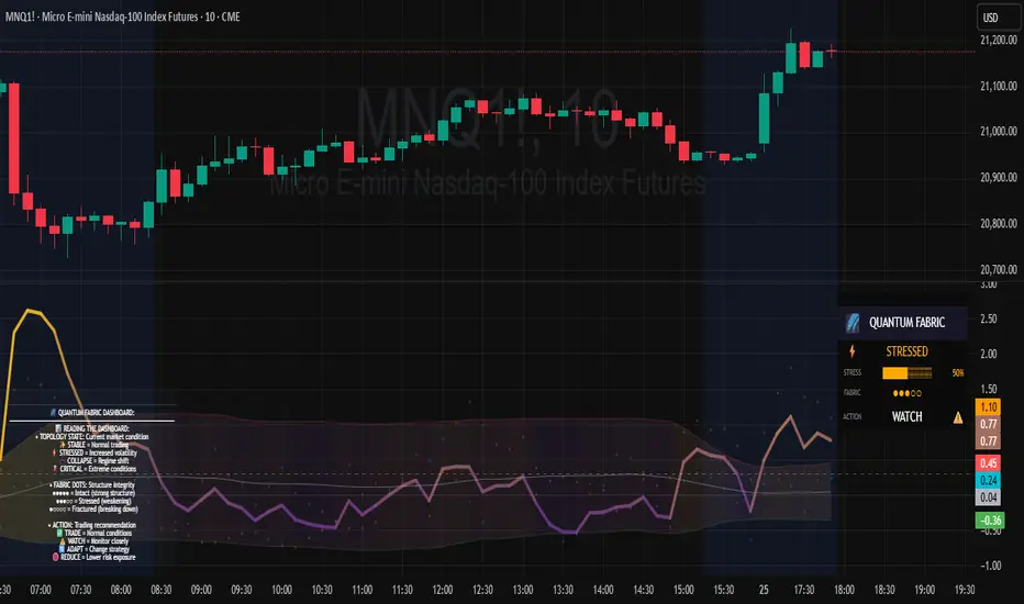
VIX Z-Score (Inverted)📘 Indicator: VIX Z-Score (Inverted) + Table
🔍 Overview
This indicator calculates the Z-Score of the VIX (Volatility Index) and inverts it to identify potential buying opportunities during periods of fear and caution during periods of extreme optimism. The Z-Score is smoothed and visually displayed alongside a dynamic info table.
⚙️ How It Works
VIX Data: The VIX (ticker: CBOE:VIX) is pulled in real time.
Z-Score Calculation:
𝑍
=
(
𝑉
𝐼
𝑋
−
mean
)
standard deviation
Z=
standard deviation
(VIX−mean)
Over a customizable lookback period (default: 50).
Inversion:
Since high VIX usually means fear (often a contrarian buying signal), we invert the Z-Score:
𝑍
inv
=
−
𝑍
Z
inv
=−Z
Smoothing:
An EMA is applied to reduce noise and false signals.
Clamping:
The Z-Score is linearly scaled and capped between +2 and -2 for easy visualization in the info table.
📊 Z-Score Table (Top-Right)
Range Interpretation Table Color
+1.5 to +2 Extreme fear → Buy zone 🟩 Green
+0.5 to +1.5 Moderate fear 🟨 Lime
–0.5 to +0.5 Neutral ⬜ Gray
–0.5 to –1.5 Growing complacency 🟧 Orange
–1.5 to –2 Extreme optimism → Caution 🟥 Red
The current Z-Score (clamped version) is shown in real time on the right-hand info panel.
🧠 How to Use It
+2 Zone (Table: Green):
Market fear is at an extreme. Historically, such conditions are contrarian bullish—possible entry zones.
–2 Zone (Table: Red):
Indicates extreme optimism and low fear. Often a signal to be cautious or take profits.
Middle range (±0.5):
Market is neutral. Avoid major decisions based solely on sentiment here.
🧪 Best Practices
Combine with price action, volume, or trend filters.
Works well on daily or 4H timeframes.
Not a standalone signal—best used to confirm or fade sentiment extremes.

Fuzzy SMA with DCTI Confirmation[FibonacciFlux]FibonacciFlux: Advanced Fuzzy Logic System with Donchian Trend Confirmation
Institutional-grade trend analysis combining adaptive Fuzzy Logic with Donchian Channel Trend Intensity for superior signal quality
Conceptual Framework & Research Foundation
FibonacciFlux represents a significant advancement in quantitative technical analysis, merging two powerful analytical methodologies: normalized fuzzy logic systems and Donchian Channel Trend Intensity (DCTI). This sophisticated indicator addresses a fundamental challenge in market analysis – the inherent imprecision of trend identification in dynamic, multi-dimensional market environments.
While traditional indicators often produce simplistic binary signals, markets exist in states of continuous, graduated transition. FibonacciFlux embraces this complexity through its implementation of fuzzy set theory, enhanced by DCTI's structural trend confirmation capabilities. The result is an indicator that provides nuanced, probabilistic trend assessment with institutional-grade signal quality.
Core Technological Components
1. Advanced Fuzzy Logic System with Percentile Normalization
At the foundation of FibonacciFlux lies a comprehensive fuzzy logic system that transforms conventional technical metrics into degrees of membership in linguistic variables:
// Fuzzy triangular membership function with robust error handling
fuzzy_triangle(val, left, center, right) =>
if na(val)
0.0
float denominator1 = math.max(1e-10, center - left)
float denominator2 = math.max(1e-10, right - center)
math.max(0.0, math.min(left == center ? val <= center ? 1.0 : 0.0 : (val - left) / denominator1,
center == right ? val >= center ? 1.0 : 0.0 : (right - val) / denominator2))
The system employs percentile-based normalization for SMA deviation – a critical innovation that enables self-calibration across different assets and market regimes:
// Percentile-based normalization for adaptive calibration
raw_diff = price_src - sma_val
diff_abs_percentile = ta.percentile_linear_interpolation(math.abs(raw_diff), normLookback, percRank) + 1e-10
normalized_diff_raw = raw_diff / diff_abs_percentile
normalized_diff = useClamping ? math.max(-clampValue, math.min(clampValue, normalized_diff_raw)) : normalized_diff_raw
This normalization approach represents a significant advancement over fixed-threshold systems, allowing the indicator to automatically adapt to varying volatility environments and maintain consistent signal quality across diverse market conditions.
2. Donchian Channel Trend Intensity (DCTI) Integration
FibonacciFlux significantly enhances fuzzy logic analysis through the integration of Donchian Channel Trend Intensity (DCTI) – a sophisticated measure of trend strength based on the relationship between short-term and long-term price extremes:
// DCTI calculation for structural trend confirmation
f_dcti(src, majorPer, minorPer, sigPer) =>
H = ta.highest(high, majorPer) // Major period high
L = ta.lowest(low, majorPer) // Major period low
h = ta.highest(high, minorPer) // Minor period high
l = ta.lowest(low, minorPer) // Minor period low
float pdiv = not na(L) ? l - L : 0 // Positive divergence (low vs major low)
float ndiv = not na(H) ? H - h : 0 // Negative divergence (major high vs high)
float divisor = pdiv + ndiv
dctiValue = divisor == 0 ? 0 : 100 * ((pdiv - ndiv) / divisor) // Normalized to -100 to +100 range
sigValue = ta.ema(dctiValue, sigPer)
DCTI provides a complementary structural perspective on market trends by quantifying the relationship between short-term and long-term price extremes. This creates a multi-dimensional analysis framework that combines adaptive deviation measurement (fuzzy SMA) with channel-based trend intensity confirmation (DCTI).
Multi-Dimensional Fuzzy Input Variables
FibonacciFlux processes four distinct technical dimensions through its fuzzy system:
Normalized SMA Deviation: Measures price displacement relative to historical volatility context
Rate of Change (ROC): Captures price momentum over configurable timeframes
Relative Strength Index (RSI): Evaluates cyclical overbought/oversold conditions
Donchian Channel Trend Intensity (DCTI): Provides structural trend confirmation through channel analysis
Each dimension is processed through comprehensive fuzzy sets that transform crisp numerical values into linguistic variables:
// Normalized SMA Deviation - Self-calibrating to volatility regimes
ndiff_LP := fuzzy_triangle(normalized_diff, norm_scale * 0.3, norm_scale * 0.7, norm_scale * 1.1)
ndiff_SP := fuzzy_triangle(normalized_diff, norm_scale * 0.05, norm_scale * 0.25, norm_scale * 0.5)
ndiff_NZ := fuzzy_triangle(normalized_diff, -norm_scale * 0.1, 0.0, norm_scale * 0.1)
ndiff_SN := fuzzy_triangle(normalized_diff, -norm_scale * 0.5, -norm_scale * 0.25, -norm_scale * 0.05)
ndiff_LN := fuzzy_triangle(normalized_diff, -norm_scale * 1.1, -norm_scale * 0.7, -norm_scale * 0.3)
// DCTI - Structural trend measurement
dcti_SP := fuzzy_triangle(dcti_val, 60.0, 85.0, 101.0) // Strong Positive Trend (> ~85)
dcti_WP := fuzzy_triangle(dcti_val, 20.0, 45.0, 70.0) // Weak Positive Trend (~30-60)
dcti_Z := fuzzy_triangle(dcti_val, -30.0, 0.0, 30.0) // Near Zero / Trendless (~+/- 20)
dcti_WN := fuzzy_triangle(dcti_val, -70.0, -45.0, -20.0) // Weak Negative Trend (~-30 - -60)
dcti_SN := fuzzy_triangle(dcti_val, -101.0, -85.0, -60.0) // Strong Negative Trend (< ~-85)
Advanced Fuzzy Rule System with DCTI Confirmation
The core intelligence of FibonacciFlux lies in its sophisticated fuzzy rule system – a structured knowledge representation that encodes expert understanding of market dynamics:
// Base Trend Rules with DCTI Confirmation
cond1 = math.min(ndiff_LP, roc_HP, rsi_M)
strength_SB := math.max(strength_SB, cond1 * (dcti_SP > 0.5 ? 1.2 : dcti_Z > 0.1 ? 0.5 : 1.0))
// DCTI Override Rules - Structural trend confirmation with momentum alignment
cond14 = math.min(ndiff_NZ, roc_HP, dcti_SP)
strength_SB := math.max(strength_SB, cond14 * 0.5)
The rule system implements 15 distinct fuzzy rules that evaluate various market conditions including:
Established Trends: Strong deviations with confirming momentum and DCTI alignment
Emerging Trends: Early deviation patterns with initial momentum and DCTI confirmation
Weakening Trends: Divergent signals between deviation, momentum, and DCTI
Reversal Conditions: Counter-trend signals with DCTI confirmation
Neutral Consolidations: Minimal deviation with low momentum and neutral DCTI
A key innovation is the weighted influence of DCTI on rule activation. When strong DCTI readings align with other indicators, rule strength is amplified (up to 1.2x). Conversely, when DCTI contradicts other indicators, rule impact is reduced (as low as 0.5x). This creates a dynamic, self-adjusting system that prioritizes high-conviction signals.
Defuzzification & Signal Generation
The final step transforms fuzzy outputs into a precise trend score through center-of-gravity defuzzification:
// Defuzzification with precise floating-point handling
denominator = strength_SB + strength_WB + strength_N + strength_WBe + strength_SBe
if denominator > 1e-10
fuzzyTrendScore := (strength_SB * STRONG_BULL + strength_WB * WEAK_BULL +
strength_N * NEUTRAL + strength_WBe * WEAK_BEAR +
strength_SBe * STRONG_BEAR) / denominator
The resulting FuzzyTrendScore ranges from -1.0 (Strong Bear) to +1.0 (Strong Bull), with critical threshold zones at ±0.3 (Weak trend) and ±0.7 (Strong trend). The histogram visualization employs intuitive color-coding for immediate trend assessment.
Strategic Applications for Institutional Trading
FibonacciFlux provides substantial advantages for sophisticated trading operations:
Multi-Timeframe Signal Confirmation: Institutional-grade signal validation across multiple technical dimensions
Trend Strength Quantification: Precise measurement of trend conviction with noise filtration
Early Trend Identification: Detection of emerging trends before traditional indicators through fuzzy pattern recognition
Adaptive Market Regime Analysis: Self-calibrating analysis across varying volatility environments
Algorithmic Strategy Integration: Well-defined numerical output suitable for systematic trading frameworks
Risk Management Enhancement: Superior signal fidelity for risk exposure optimization
Customization Parameters
FibonacciFlux offers extensive customization to align with specific trading mandates and market conditions:
Fuzzy SMA Settings: Configure baseline trend identification parameters including SMA, ROC, and RSI lengths
Normalization Settings: Fine-tune the self-calibration mechanism with adjustable lookback period, percentile rank, and optional clamping
DCTI Parameters: Optimize trend structure confirmation with adjustable major/minor periods and signal smoothing
Visualization Controls: Customize display transparency for optimal chart integration
These parameters enable precise calibration for different asset classes, timeframes, and market regimes while maintaining the core analytical framework.
Implementation Notes
For optimal implementation, consider the following guidance:
Higher timeframes (4H+) benefit from increased normalization lookback (800+) for stability
Volatile assets may require adjusted clamping values (2.5-4.0) for optimal signal sensitivity
DCTI parameters should be aligned with chart timeframe (higher timeframes require increased major/minor periods)
The indicator performs exceptionally well as a trend filter for systematic trading strategies
Acknowledgments
FibonacciFlux builds upon the pioneering work of Donovan Wall in Donchian Channel Trend Intensity analysis. The normalization approach draws inspiration from percentile-based statistical techniques in quantitative finance. This indicator is shared for educational and analytical purposes under Attribution-NonCommercial-ShareAlike 4.0 International (CC BY-NC-SA 4.0) license.
Past performance does not guarantee future results. All trading involves risk. This indicator should be used as one component of a comprehensive analysis framework.
Shout out @DonovanWall
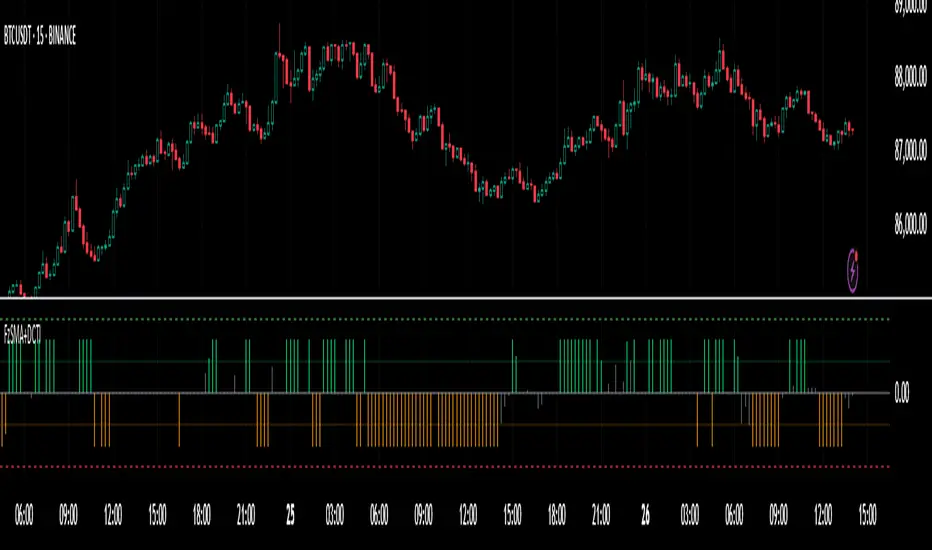
Hurst-Based Trend Persistence w/Poisson Prediction
---
# **Hurst-Based Trend Persistence w/ Poisson Prediction**
## **Introduction**
The **Hurst-Based Trend Persistence with Poisson Prediction** is a **statistically-driven trend-following oscillator** that provides traders with **a structured approach to identifying trend strength, persistence, and potential reversals**.
This indicator combines:
- **Hurst Exponent Analysis** (to measure how persistent or mean-reverting price action is).
- **Color-Coded Trend Detection** (to highlight bullish and bearish conditions).
- **Poisson-Based Trend Reversal Probability Projection** (to anticipate when a trend is likely to end based on statistical models).
By integrating **fractal market theory (Hurst exponent)** with **Poisson probability distributions**, this indicator gives traders a **probability-weighted view of trend duration** while dynamically adapting to market volatility.
---
## **Simplified Explanation (How to Read the Indicator at a Glance)**
1. **If the oscillator line is going up → The trend is strong.**
2. **If the oscillator line is going down → The trend is weakening.**
3. **If the color shifts from red to green (or vice versa), a trend shift has occurred.**
- **Strong trends can change color without weakening** (meaning a bullish or bearish move can remain powerful even as the trend shifts).
4. **A weakening trend does NOT necessarily mean a reversal is coming.**
- The trend may slow down but continue in the same direction.
5. **A strong trend does NOT guarantee it will last.**
- Even a powerful move can **suddenly reverse**, which is why the **Poisson-based background shading** helps anticipate probabilities of change.
---
## **How to Use the Indicator**
### **1. Understanding the Rolling Hurst-Based Trend Oscillator (Main Line)**
The **oscillator line** is based on the **Hurst exponent (H)**, which quantifies whether price movements are:
- **Trending** (values above 0 → momentum-driven, persistent trends).
- **Mean-reverting** (values below 0 → price action is choppy, likely to revert to the mean).
- **Neutral (Random Walk)** (values around 0 → price behaves like a purely stochastic process).
#### **Interpreting the Oscillator:**
- **H > 0.5 → Persistent Trends:**
- Price moves tend to sustain in one direction for longer periods.
- Example: Strong uptrends in bull markets.
- **H < 0.5 → Mean-Reverting Behavior:**
- Price has a tendency to revert back to its mean.
- Example: Sideways markets or fading momentum.
- **H ≈ 0.5 → Random Walk:**
- No clear trend; price is unpredictable.
A **gray dashed horizontal line at 0** serves as a **baseline**, helping traders quickly assess whether the market is **favoring trends or mean reversion**.
---
### **2. Color-Coded Trend Signal (Visual Confirmation of Trend Shifts)**
The oscillator **changes color** based on **price slope** over the lookback period:
- **🟢 Green → Uptrend (Price Increasing)**
- Price is rising relative to the selected lookback period.
- Suggests sustained bullish pressure.
- **🔴 Red → Downtrend (Price Decreasing)**
- Price is falling relative to the selected lookback period.
- Suggests sustained bearish pressure.
#### **How to Use This in Trading**
✔ **Stay in trends until a color change occurs.**
✔ **Use color changes as confirmation for trend reversals.**
✔ **Avoid counter-trend trades when the oscillator remains strongly colored.**
---
### **3. Poisson-Based Trend Reversal Projection (Anticipating Future Shifts)**
The **shaded orange background** represents a **Poisson-based probability estimation** of when the trend is likely to reverse.
- **Darker Orange = Higher Probability of Trend Reversal**
- **Lighter Orange / No Shade = Low Probability of Immediate Reversal**
💡 **The idea behind this model:**
✔ Trends **don’t last forever**, and their duration follows **statistical patterns**.
✔ By calculating the **average historical trend duration**, the indicator predicts **how likely a trend shift is at any given time**.
✔ The **Poisson probability function** is applied to determine the **expected likelihood of a reversal as time progresses**.
---
## **Mathematical Foundations of the Indicator**
This indicator is based on **two primary statistical models**:
### **1. Hurst Exponent & Trend Persistence (Fractal Market Theory)**
- The **Hurst exponent (H)** measures **autocorrelation** in price movements.
- If past trends **persist**, H will be **above 0.5** (meaning trend-following strategies are favorable).
- If past trends tend to **mean-revert**, H will be **below 0.5** (meaning reversal strategies are more effective).
- The **Rolling Hurst Oscillator** calculates this exponent over a moving window to track real-time trend conditions.
#### **Formula Breakdown (Simplified for Traders)**
The Hurst exponent (H) is derived using the **Rescaled Range (R/S) Analysis**:
\
Where:
- **R** = **Range** (difference between max cumulative deviation and min cumulative deviation).
- **S** = **Standard deviation** of price fluctuations.
- **Lookback** = The number of periods analyzed.
---
### **2. Poisson-Based Trend Reversal Probability (Stochastic Process Modeling)**
The **Poisson process** is a **probabilistic model used for estimating time-based events**, applied here to **predict trend reversals based on past trend durations**.
#### **How It Works**
- The indicator **tracks trend durations** (the time between color changes).
- A **Poisson rate parameter (λ)** is computed as:
\
- The **probability of a reversal at any given time (t)** is estimated using:
\
- **As t increases (trend continues), the probability of reversal rises**.
- The indicator **shades the background based on this probability**, visually displaying the likelihood of a **trend shift**.
---
## **Dynamic Adaptation to Market Conditions**
✔ **Volatility-Adjusted Trend Shifts:**
- A **custom volatility calculation** dynamically adjusts the **minimum trend duration** required before a trend shift is recognized.
- **Higher volatility → Requires longer confirmation before switching trend color.**
- **Lower volatility → Allows faster trend shifts.**
✔ **Adaptive Poisson Weighting:**
- **Recent trends are weighted more heavily** using an exponential decay function:
- **Decay Factor (0.618 by default)** prioritizes **recent intervals** while still considering historical trends.
- This ensures the model adapts to changing market conditions.
---
## **Key Takeaways for Traders**
✅ **Identify Persistent Trends vs. Mean Reversion:**
- Use the oscillator line to determine whether the market favors **trend-following or counter-trend strategies**.
✅ **Visual Trend Confirmation via Color Coding:**
- **Green = Uptrend**, **Red = Downtrend**.
- Trend changes help confirm **entry and exit points**.
✅ **Anticipate Trend Reversals Using Probability Models:**
- The **Poisson projection** provides a **statistical edge** in **timing exits before trends reverse**.
✅ **Adapt to Market Volatility Automatically:**
- Dynamic **volatility scaling** ensures the indicator remains effective in **both high and low volatility environments**.
Happy trading and enjoy!

Advanced Multi-Timeframe Trading System (Risk Managed)Description:
This strategy is an original approach that combines two main analytical components to identify potential trade opportunities while simulating realistic trading conditions:
1. Market Trend Analysis via an Approximate Hurst Exponent
• What It Does:
The strategy computes a rough measure of market trending using an approximate Hurst exponent. A value above 0.5 suggests persistent, trending behavior, while a value below 0.5 indicates a tendency toward mean-reversion.
• How It’s Used:
The Hurst exponent is calculated on both the chart’s current timeframe and a higher timeframe (default: Daily) to capture both local and broader market dynamics.
2. Fibonacci Retracement Levels
• What It Does:
Using daily high and low data from a selected timeframe (default: Daily), the script computes key Fibonacci retracement levels.
• How It’s Used:
• The 61.8% level (Golden Ratio) serves as a key threshold:
• A long entry is signaled when the price crosses above this level if the daily Hurst exponent confirms a trending market.
• The 38.2% level is used to identify short-entry opportunities when the price crosses below it and the daily Hurst indicates non-trending conditions.
Signal Logic:
• Long Entry:
When the price crosses above the 61.8% Fibonacci level (Golden Ratio) and the daily Hurst exponent is greater than 0.5, suggesting a trending market.
• Short Entry:
When the price crosses below the 38.2% Fibonacci level and the daily Hurst exponent is less than 0.5, indicating a less trending or potentially reversing market.
Risk Management & Trade Execution:
• Stop-Loss:
Each trade is risk-managed with a stop-loss set at 2% below (for longs) or above (for shorts) the entry price. This ensures that no single trade risks more than a small, sustainable portion of the account.
• Take Profit:
A take profit order targets a risk-reward ratio of 1:2 (i.e., the target profit is twice the amount risked).
• Position Sizing:
Trades are executed with a fixed position size equal to 10% of account equity.
• Trade Frequency Limits:
• Daily Limit: A maximum of 5 trades per day
• Overall Limit: No more than 510 trades during the backtesting period (e.g., since 2019)
These limits are imposed to simulate realistic trading frequency and to avoid overtrading in backtest results.
Backtesting Parameters:
• Initial Capital: $10,000
• Commission: 0.1% per trade
• Slippage: 1 tick per bar
These settings aim to reflect the conditions faced by the average trader and help ensure that the backtesting results are realistic and not misleading.
Chart Overlays & Visual Aids:
• Fibonacci Levels:
The key Fibonacci retracement levels are plotted on the chart, and the zone between the 61.8% and 38.2% levels is highlighted to show a key retracement area.
• Market Trend Background:
The chart background is tinted green when the daily Hurst exponent indicates a trending market (value > 0.5) and red otherwise.
• Information Table:
An on-chart table displays key parameters such as the current Hurst exponent, daily Hurst value, the number of trades executed today, and the global trade count.
Disclaimer:
Past performance is not indicative of future results. This strategy is experimental and provided solely for educational purposes. It is essential that you backtest and paper trade using your own settings before considering any live deployment. The Hurst exponent calculation is an approximation and should be interpreted as a rough gauge of market behavior. Adjust the parameters and risk management settings according to your personal risk tolerance and market conditions.
Additional Notes:
• Originality & Usefulness:
This script is an original mashup that combines trend analysis with Fibonacci retracement methods. The description above explains how these components work together to provide trading signals.
• Realistic Results:
The strategy uses realistic account sizes, commission rates, slippage, and risk management rules to generate backtesting results that are representative of real-world trading.
• Educational Purpose:
This script is intended to support the TradingView community by offering insights into combining multiple analysis techniques in one strategy. It is not a “get-rich-quick” system but rather an educational tool to help traders understand risk management and trade signal logic.
By using this script, you acknowledge that trading involves risk and that you are responsible for testing and adjusting the strategy to fit your own trading environment. This publication is fully open source, and any modifications should include proper attribution if significant portions of the code are reused.