Dynamic Equity Allocation Model//@version=6
indicator('Dynamic Equity Allocation Model', shorttitle = 'DEAM', overlay = false, precision = 1, scale = scale.right, max_bars_back = 500)
// DYNAMIC EQUITY ALLOCATION MODEL
// Quantitative framework for dynamic portfolio allocation between stocks and cash.
// Analyzes five dimensions: market regime, risk metrics, valuation, sentiment,
// and macro conditions to generate allocation recommendations (0-100% equity).
//
// Uses real-time data from TradingView including fundamentals (P/E, ROE, ERP),
// volatility indicators (VIX), credit spreads, yield curves, and market structure.
// INPUT PARAMETERS
group1 = 'Model Configuration'
model_type = input.string('Adaptive', 'Allocation Model Type', options = , group = group1, tooltip = 'Conservative: Slower to increase equity, Aggressive: Faster allocation changes, Adaptive: Dynamic based on regime')
use_crisis_detection = input.bool(true, 'Enable Crisis Detection System', group = group1, tooltip = 'Automatic detection and response to crisis conditions')
use_regime_model = input.bool(true, 'Use Market Regime Detection', group = group1, tooltip = 'Identify Bull/Bear/Crisis regimes for dynamic allocation')
group2 = 'Portfolio Risk Management'
target_portfolio_volatility = input.float(12.0, 'Target Portfolio Volatility (%)', minval = 3, maxval = 20, step = 0.5, group = group2, tooltip = 'Target portfolio volatility (Cash reduces volatility: 50% Equity = ~10% vol, 100% Equity = ~20% vol)')
max_portfolio_drawdown = input.float(15.0, 'Maximum Portfolio Drawdown (%)', minval = 5, maxval = 35, step = 2.5, group = group2, tooltip = 'Maximum acceptable PORTFOLIO drawdown (not market drawdown - portfolio with cash has lower drawdown)')
enable_portfolio_risk_scaling = input.bool(true, 'Enable Portfolio Risk Scaling', group = group2, tooltip = 'Scale allocation based on actual portfolio risk characteristics (recommended)')
risk_lookback = input.int(252, 'Risk Calculation Period (Days)', minval = 60, maxval = 504, group = group2, tooltip = 'Period for calculating volatility and risk metrics')
group3 = 'Component Weights (Total = 100%)'
w_regime = input.float(35.0, 'Market Regime Weight (%)', minval = 0, maxval = 100, step = 5, group = group3)
w_risk = input.float(25.0, 'Risk Metrics Weight (%)', minval = 0, maxval = 100, step = 5, group = group3)
w_valuation = input.float(20.0, 'Valuation Weight (%)', minval = 0, maxval = 100, step = 5, group = group3)
w_sentiment = input.float(15.0, 'Sentiment Weight (%)', minval = 0, maxval = 100, step = 5, group = group3)
w_macro = input.float(5.0, 'Macro Weight (%)', minval = 0, maxval = 100, step = 5, group = group3)
group4 = 'Crisis Detection Thresholds'
crisis_vix_threshold = input.float(40, 'Crisis VIX Level', minval = 30, maxval = 80, group = group4, tooltip = 'VIX level indicating crisis conditions (COVID peaked at 82)')
crisis_drawdown_threshold = input.float(15, 'Crisis Drawdown Threshold (%)', minval = 10, maxval = 30, group = group4, tooltip = 'Market drawdown indicating crisis conditions')
crisis_credit_spread = input.float(500, 'Crisis Credit Spread (bps)', minval = 300, maxval = 1000, group = group4, tooltip = 'High yield spread indicating crisis conditions')
group5 = 'Display Settings'
show_components = input.bool(false, 'Show Component Breakdown', group = group5, tooltip = 'Display individual component analysis lines')
show_regime_background = input.bool(true, 'Show Dynamic Background', group = group5, tooltip = 'Color background based on allocation signals')
show_reference_lines = input.bool(false, 'Show Reference Lines', group = group5, tooltip = 'Display allocation percentage reference lines')
show_dashboard = input.bool(true, 'Show Analytics Dashboard', group = group5, tooltip = 'Display comprehensive analytics table')
show_confidence_bands = input.bool(false, 'Show Confidence Bands', group = group5, tooltip = 'Display uncertainty quantification bands')
smoothing_period = input.int(3, 'Smoothing Period', minval = 1, maxval = 10, group = group5, tooltip = 'Smoothing to reduce allocation noise')
background_intensity = input.int(95, 'Background Intensity (%)', minval = 90, maxval = 99, group = group5, tooltip = 'Higher values = more transparent background')
// Styling Options
color_scheme = input.string('EdgeTools', 'Color Theme', options = , group = 'Appearance', tooltip = 'Professional color themes')
use_dark_mode = input.bool(true, 'Optimize for Dark Theme', group = 'Appearance')
main_line_width = input.int(3, 'Main Line Width', minval = 1, maxval = 5, group = 'Appearance')
// DATA RETRIEVAL
// Market Data
sp500 = request.security('SPY', timeframe.period, close)
sp500_high = request.security('SPY', timeframe.period, high)
sp500_low = request.security('SPY', timeframe.period, low)
sp500_volume = request.security('SPY', timeframe.period, volume)
// Volatility Indicators
vix = request.security('VIX', timeframe.period, close)
vix9d = request.security('VIX9D', timeframe.period, close)
vxn = request.security('VXN', timeframe.period, close)
// Fixed Income and Credit
us2y = request.security('US02Y', timeframe.period, close)
us10y = request.security('US10Y', timeframe.period, close)
us3m = request.security('US03MY', timeframe.period, close)
hyg = request.security('HYG', timeframe.period, close)
lqd = request.security('LQD', timeframe.period, close)
tlt = request.security('TLT', timeframe.period, close)
// Safe Haven Assets
gold = request.security('GLD', timeframe.period, close)
usd = request.security('DXY', timeframe.period, close)
yen = request.security('JPYUSD', timeframe.period, close)
// Financial data with fallback values
get_financial_data(symbol, fin_id, period, fallback) =>
data = request.financial(symbol, fin_id, period, ignore_invalid_symbol = true)
na(data) ? fallback : data
// SPY fundamental metrics
spy_earnings_per_share = get_financial_data('AMEX:SPY', 'EARNINGS_PER_SHARE_BASIC', 'TTM', 20.0)
spy_operating_earnings_yield = get_financial_data('AMEX:SPY', 'OPERATING_EARNINGS_YIELD', 'FY', 4.5)
spy_dividend_yield = get_financial_data('AMEX:SPY', 'DIVIDENDS_YIELD', 'FY', 1.8)
spy_buyback_yield = get_financial_data('AMEX:SPY', 'BUYBACK_YIELD', 'FY', 2.0)
spy_net_margin = get_financial_data('AMEX:SPY', 'NET_MARGIN', 'TTM', 12.0)
spy_debt_to_equity = get_financial_data('AMEX:SPY', 'DEBT_TO_EQUITY', 'FY', 0.5)
spy_return_on_equity = get_financial_data('AMEX:SPY', 'RETURN_ON_EQUITY', 'FY', 15.0)
spy_free_cash_flow = get_financial_data('AMEX:SPY', 'FREE_CASH_FLOW', 'TTM', 100000000)
spy_ebitda = get_financial_data('AMEX:SPY', 'EBITDA', 'TTM', 200000000)
spy_pe_forward = get_financial_data('AMEX:SPY', 'PRICE_EARNINGS_FORWARD', 'FY', 18.0)
spy_total_debt = get_financial_data('AMEX:SPY', 'TOTAL_DEBT', 'FY', 500000000)
spy_total_equity = get_financial_data('AMEX:SPY', 'TOTAL_EQUITY', 'FY', 1000000000)
spy_enterprise_value = get_financial_data('AMEX:SPY', 'ENTERPRISE_VALUE', 'FY', 30000000000)
spy_revenue_growth = get_financial_data('AMEX:SPY', 'REVENUE_ONE_YEAR_GROWTH', 'TTM', 5.0)
// Market Breadth Indicators
nya = request.security('NYA', timeframe.period, close)
rut = request.security('IWM', timeframe.period, close)
// Sector Performance
xlk = request.security('XLK', timeframe.period, close)
xlu = request.security('XLU', timeframe.period, close)
xlf = request.security('XLF', timeframe.period, close)
// MARKET REGIME DETECTION
// Calculate Market Trend
sma_20 = ta.sma(sp500, 20)
sma_50 = ta.sma(sp500, 50)
sma_200 = ta.sma(sp500, 200)
ema_10 = ta.ema(sp500, 10)
// Market Structure Score
trend_strength = 0.0
trend_strength := trend_strength + (sp500 > sma_20 ? 1 : -1)
trend_strength := trend_strength + (sp500 > sma_50 ? 1 : -1)
trend_strength := trend_strength + (sp500 > sma_200 ? 2 : -2)
trend_strength := trend_strength + (sma_50 > sma_200 ? 2 : -2)
// Volatility Regime
returns = math.log(sp500 / sp500 )
realized_vol_20d = ta.stdev(returns, 20) * math.sqrt(252) * 100
realized_vol_60d = ta.stdev(returns, 60) * math.sqrt(252) * 100
ewma_vol = ta.ema(math.pow(returns, 2), 20)
realized_vol = math.sqrt(ewma_vol * 252) * 100
vol_premium = vix - realized_vol
// Drawdown Calculation
running_max = ta.highest(sp500, risk_lookback)
current_drawdown = (running_max - sp500) / running_max * 100
// Regime Score
regime_score = 0.0
// Trend Component (40%)
if trend_strength >= 4
regime_score := regime_score + 40
regime_score
else if trend_strength >= 2
regime_score := regime_score + 30
regime_score
else if trend_strength >= 0
regime_score := regime_score + 20
regime_score
else if trend_strength >= -2
regime_score := regime_score + 10
regime_score
else
regime_score := regime_score + 0
regime_score
// Volatility Component (30%)
if vix < 15
regime_score := regime_score + 30
regime_score
else if vix < 20
regime_score := regime_score + 25
regime_score
else if vix < 25
regime_score := regime_score + 15
regime_score
else if vix < 35
regime_score := regime_score + 5
regime_score
else
regime_score := regime_score + 0
regime_score
// Drawdown Component (30%)
if current_drawdown < 3
regime_score := regime_score + 30
regime_score
else if current_drawdown < 7
regime_score := regime_score + 20
regime_score
else if current_drawdown < 12
regime_score := regime_score + 10
regime_score
else if current_drawdown < 20
regime_score := regime_score + 5
regime_score
else
regime_score := regime_score + 0
regime_score
// Classify Regime
market_regime = regime_score >= 80 ? 'Strong Bull' : regime_score >= 60 ? 'Bull Market' : regime_score >= 40 ? 'Neutral' : regime_score >= 20 ? 'Correction' : regime_score >= 10 ? 'Bear Market' : 'Crisis'
// RISK-BASED ALLOCATION
// Calculate Market Risk
parkinson_hl = math.log(sp500_high / sp500_low)
parkinson_vol = parkinson_hl / (2 * math.sqrt(math.log(2))) * math.sqrt(252) * 100
garman_klass_vol = math.sqrt((0.5 * math.pow(math.log(sp500_high / sp500_low), 2) - (2 * math.log(2) - 1) * math.pow(math.log(sp500 / sp500 ), 2)) * 252) * 100
market_volatility_20d = math.max(ta.stdev(returns, 20) * math.sqrt(252) * 100, parkinson_vol)
market_volatility_60d = ta.stdev(returns, 60) * math.sqrt(252) * 100
market_drawdown = current_drawdown
// Initialize risk allocation
risk_allocation = 50.0
if enable_portfolio_risk_scaling
// Volatility-based allocation
vol_based_allocation = target_portfolio_volatility / math.max(market_volatility_20d, 5.0) * 100
vol_based_allocation := math.max(0, math.min(100, vol_based_allocation))
// Drawdown-based allocation
dd_based_allocation = 100.0
if market_drawdown > 1.0
dd_based_allocation := max_portfolio_drawdown / market_drawdown * 100
dd_based_allocation := math.max(0, math.min(100, dd_based_allocation))
dd_based_allocation
// Combine (conservative)
risk_allocation := math.min(vol_based_allocation, dd_based_allocation)
// Dynamic adjustment
current_equity_estimate = 50.0
estimated_portfolio_vol = current_equity_estimate / 100 * market_volatility_20d
estimated_portfolio_dd = current_equity_estimate / 100 * market_drawdown
vol_utilization = estimated_portfolio_vol / target_portfolio_volatility
dd_utilization = estimated_portfolio_dd / max_portfolio_drawdown
risk_utilization = math.max(vol_utilization, dd_utilization)
risk_adjustment_factor = 1.0
if risk_utilization > 1.0
risk_adjustment_factor := math.exp(-0.5 * (risk_utilization - 1.0))
risk_adjustment_factor := math.max(0.5, risk_adjustment_factor)
risk_adjustment_factor
else if risk_utilization < 0.9
risk_adjustment_factor := 1.0 + 0.2 * math.log(1.0 / risk_utilization)
risk_adjustment_factor := math.min(1.3, risk_adjustment_factor)
risk_adjustment_factor
risk_allocation := risk_allocation * risk_adjustment_factor
risk_allocation
else
vol_scalar = target_portfolio_volatility / math.max(market_volatility_20d, 10)
vol_scalar := math.min(1.5, math.max(0.2, vol_scalar))
drawdown_penalty = 0.0
if current_drawdown > max_portfolio_drawdown
drawdown_penalty := (current_drawdown - max_portfolio_drawdown) / max_portfolio_drawdown
drawdown_penalty := math.min(1.0, drawdown_penalty)
drawdown_penalty
risk_allocation := 100 * vol_scalar * (1 - drawdown_penalty)
risk_allocation
risk_allocation := math.max(0, math.min(100, risk_allocation))
// VALUATION ANALYSIS
// Valuation Metrics
actual_pe_ratio = spy_earnings_per_share > 0 ? sp500 / spy_earnings_per_share : spy_pe_forward
actual_earnings_yield = nz(spy_operating_earnings_yield, 0) > 0 ? spy_operating_earnings_yield : 100 / actual_pe_ratio
total_shareholder_yield = spy_dividend_yield + spy_buyback_yield
// Equity Risk Premium (multi-method calculation)
method1_erp = actual_earnings_yield - us10y
method2_erp = actual_earnings_yield + spy_buyback_yield - us10y
payout_ratio = spy_dividend_yield > 0 and actual_earnings_yield > 0 ? spy_dividend_yield / actual_earnings_yield : 0.4
sustainable_growth = spy_return_on_equity * (1 - payout_ratio) / 100
method3_erp = spy_dividend_yield + sustainable_growth * 100 - us10y
implied_growth = spy_revenue_growth * 0.7
method4_erp = total_shareholder_yield + implied_growth - us10y
equity_risk_premium = method1_erp * 0.35 + method2_erp * 0.30 + method3_erp * 0.20 + method4_erp * 0.15
ev_ebitda_ratio = spy_enterprise_value > 0 and spy_ebitda > 0 ? spy_enterprise_value / spy_ebitda : 15.0
debt_equity_health = spy_debt_to_equity < 1.0 ? 1.2 : spy_debt_to_equity < 2.0 ? 1.0 : 0.8
// Valuation Score
base_valuation_score = 50.0
if equity_risk_premium > 4
base_valuation_score := 95
base_valuation_score
else if equity_risk_premium > 3
base_valuation_score := 85
base_valuation_score
else if equity_risk_premium > 2
base_valuation_score := 70
base_valuation_score
else if equity_risk_premium > 1
base_valuation_score := 55
base_valuation_score
else if equity_risk_premium > 0
base_valuation_score := 40
base_valuation_score
else if equity_risk_premium > -1
base_valuation_score := 25
base_valuation_score
else
base_valuation_score := 10
base_valuation_score
growth_adjustment = spy_revenue_growth > 10 ? 10 : spy_revenue_growth > 5 ? 5 : 0
margin_adjustment = spy_net_margin > 15 ? 5 : spy_net_margin < 8 ? -5 : 0
roe_adjustment = spy_return_on_equity > 20 ? 5 : spy_return_on_equity < 10 ? -5 : 0
valuation_score = base_valuation_score + growth_adjustment + margin_adjustment + roe_adjustment
valuation_score := math.max(0, math.min(100, valuation_score * debt_equity_health))
// SENTIMENT ANALYSIS
// VIX Term Structure
vix_term_structure = vix9d > 0 ? vix / vix9d : 1
backwardation = vix_term_structure > 1.05
steep_backwardation = vix_term_structure > 1.15
// Safe Haven Flows
gold_momentum = ta.roc(gold, 20)
dollar_momentum = ta.roc(usd, 20)
yen_momentum = ta.roc(yen, 20)
treasury_momentum = ta.roc(tlt, 20)
safe_haven_flow = gold_momentum * 0.3 + treasury_momentum * 0.3 + dollar_momentum * 0.25 + yen_momentum * 0.15
// Advanced Sentiment Analysis
vix_percentile = ta.percentrank(vix, 252)
vix_zscore = (vix - ta.sma(vix, 252)) / ta.stdev(vix, 252)
vix_momentum = ta.roc(vix, 5)
vvix_proxy = ta.stdev(vix_momentum, 20) * math.sqrt(252)
risk_reversal_proxy = (vix - realized_vol) / realized_vol
// Sentiment Score
base_sentiment = 50.0
vix_adjustment = 0.0
if vix_zscore < -1.5
vix_adjustment := 40
vix_adjustment
else if vix_zscore < -0.5
vix_adjustment := 20
vix_adjustment
else if vix_zscore < 0.5
vix_adjustment := 0
vix_adjustment
else if vix_zscore < 1.5
vix_adjustment := -20
vix_adjustment
else
vix_adjustment := -40
vix_adjustment
term_structure_adjustment = backwardation ? -15 : steep_backwardation ? -30 : 5
vvix_adjustment = vvix_proxy > 2.0 ? -10 : vvix_proxy < 1.0 ? 10 : 0
sentiment_score = base_sentiment + vix_adjustment + term_structure_adjustment + vvix_adjustment
sentiment_score := math.max(0, math.min(100, sentiment_score))
// MACRO ANALYSIS
// Yield Curve
yield_spread_2_10 = us10y - us2y
yield_spread_3m_10 = us10y - us3m
// Credit Conditions
hyg_return = ta.roc(hyg, 20)
lqd_return = ta.roc(lqd, 20)
tlt_return = ta.roc(tlt, 20)
hyg_duration = 4.0
lqd_duration = 8.0
tlt_duration = 17.0
hyg_log_returns = math.log(hyg / hyg )
lqd_log_returns = math.log(lqd / lqd )
hyg_volatility = ta.stdev(hyg_log_returns, 20) * math.sqrt(252)
lqd_volatility = ta.stdev(lqd_log_returns, 20) * math.sqrt(252)
hyg_yield_proxy = -math.log(hyg / hyg ) * 100
lqd_yield_proxy = -math.log(lqd / lqd ) * 100
tlt_yield = us10y
hyg_spread = (hyg_yield_proxy - tlt_yield) * 100
lqd_spread = (lqd_yield_proxy - tlt_yield) * 100
hyg_distance = (hyg - ta.lowest(hyg, 252)) / (ta.highest(hyg, 252) - ta.lowest(hyg, 252))
lqd_distance = (lqd - ta.lowest(lqd, 252)) / (ta.highest(lqd, 252) - ta.lowest(lqd, 252))
default_risk_proxy = 2.0 - (hyg_distance + lqd_distance)
credit_spread = hyg_spread * 0.5 + (hyg_volatility - lqd_volatility) * 1000 * 0.3 + default_risk_proxy * 200 * 0.2
credit_spread := math.max(50, credit_spread)
credit_market_health = hyg_return > lqd_return ? 1 : -1
flight_to_quality = tlt_return > (hyg_return + lqd_return) / 2
// Macro Score
macro_score = 50.0
yield_curve_score = 0
if yield_spread_2_10 > 1.5 and yield_spread_3m_10 > 2
yield_curve_score := 40
yield_curve_score
else if yield_spread_2_10 > 0.5 and yield_spread_3m_10 > 1
yield_curve_score := 30
yield_curve_score
else if yield_spread_2_10 > 0 and yield_spread_3m_10 > 0
yield_curve_score := 20
yield_curve_score
else if yield_spread_2_10 < 0 or yield_spread_3m_10 < 0
yield_curve_score := 10
yield_curve_score
else
yield_curve_score := 5
yield_curve_score
credit_conditions_score = 0
if credit_spread < 200 and not flight_to_quality
credit_conditions_score := 30
credit_conditions_score
else if credit_spread < 400 and credit_market_health > 0
credit_conditions_score := 20
credit_conditions_score
else if credit_spread < 600
credit_conditions_score := 15
credit_conditions_score
else if credit_spread < 1000
credit_conditions_score := 10
credit_conditions_score
else
credit_conditions_score := 0
credit_conditions_score
financial_stability_score = 0
if spy_debt_to_equity < 0.5 and spy_return_on_equity > 15
financial_stability_score := 20
financial_stability_score
else if spy_debt_to_equity < 1.0 and spy_return_on_equity > 10
financial_stability_score := 15
financial_stability_score
else if spy_debt_to_equity < 1.5
financial_stability_score := 10
financial_stability_score
else
financial_stability_score := 5
financial_stability_score
macro_score := yield_curve_score + credit_conditions_score + financial_stability_score
macro_score := math.max(0, math.min(100, macro_score))
// CRISIS DETECTION
crisis_indicators = 0
if vix > crisis_vix_threshold
crisis_indicators := crisis_indicators + 1
crisis_indicators
if vix > 60
crisis_indicators := crisis_indicators + 2
crisis_indicators
if current_drawdown > crisis_drawdown_threshold
crisis_indicators := crisis_indicators + 1
crisis_indicators
if current_drawdown > 25
crisis_indicators := crisis_indicators + 1
crisis_indicators
if credit_spread > crisis_credit_spread
crisis_indicators := crisis_indicators + 1
crisis_indicators
sp500_roc_5 = ta.roc(sp500, 5)
tlt_roc_5 = ta.roc(tlt, 5)
if sp500_roc_5 < -10 and tlt_roc_5 < -5
crisis_indicators := crisis_indicators + 2
crisis_indicators
volume_spike = sp500_volume > ta.sma(sp500_volume, 20) * 2
sp500_roc_1 = ta.roc(sp500, 1)
if volume_spike and sp500_roc_1 < -3
crisis_indicators := crisis_indicators + 1
crisis_indicators
is_crisis = crisis_indicators >= 3
is_severe_crisis = crisis_indicators >= 5
// FINAL ALLOCATION CALCULATION
// Convert regime to base allocation
regime_allocation = market_regime == 'Strong Bull' ? 100 : market_regime == 'Bull Market' ? 80 : market_regime == 'Neutral' ? 60 : market_regime == 'Correction' ? 40 : market_regime == 'Bear Market' ? 20 : 0
// Normalize weights
total_weight = w_regime + w_risk + w_valuation + w_sentiment + w_macro
w_regime_norm = w_regime / total_weight
w_risk_norm = w_risk / total_weight
w_valuation_norm = w_valuation / total_weight
w_sentiment_norm = w_sentiment / total_weight
w_macro_norm = w_macro / total_weight
// Calculate Weighted Allocation
weighted_allocation = regime_allocation * w_regime_norm + risk_allocation * w_risk_norm + valuation_score * w_valuation_norm + sentiment_score * w_sentiment_norm + macro_score * w_macro_norm
// Apply Crisis Override
if use_crisis_detection
if is_severe_crisis
weighted_allocation := math.min(weighted_allocation, 10)
weighted_allocation
else if is_crisis
weighted_allocation := math.min(weighted_allocation, 25)
weighted_allocation
// Model Type Adjustment
model_adjustment = 0.0
if model_type == 'Conservative'
model_adjustment := -10
model_adjustment
else if model_type == 'Aggressive'
model_adjustment := 10
model_adjustment
else if model_type == 'Adaptive'
recent_return = (sp500 - sp500 ) / sp500 * 100
if recent_return > 5
model_adjustment := 5
model_adjustment
else if recent_return < -5
model_adjustment := -5
model_adjustment
// Apply adjustment and bounds
final_allocation = weighted_allocation + model_adjustment
final_allocation := math.max(0, math.min(100, final_allocation))
// Smooth allocation
smoothed_allocation = ta.sma(final_allocation, smoothing_period)
// Calculate portfolio risk metrics (only for internal alerts)
actual_portfolio_volatility = smoothed_allocation / 100 * market_volatility_20d
actual_portfolio_drawdown = smoothed_allocation / 100 * current_drawdown
// VISUALIZATION
// Color definitions
var color primary_color = #2196F3
var color bullish_color = #4CAF50
var color bearish_color = #FF5252
var color neutral_color = #808080
var color text_color = color.white
var color bg_color = #000000
var color table_bg_color = #1E1E1E
var color header_bg_color = #2D2D2D
switch color_scheme // Apply color scheme
'Gold' =>
primary_color := use_dark_mode ? #FFD700 : #DAA520
bullish_color := use_dark_mode ? #FFA500 : #FF8C00
bearish_color := use_dark_mode ? #FF5252 : #D32F2F
neutral_color := use_dark_mode ? #C0C0C0 : #808080
text_color := use_dark_mode ? color.white : color.black
bg_color := use_dark_mode ? #000000 : #FFFFFF
table_bg_color := use_dark_mode ? #1A1A00 : #FFFEF0
header_bg_color := use_dark_mode ? #2D2600 : #F5F5DC
header_bg_color
'EdgeTools' =>
primary_color := use_dark_mode ? #4682B4 : #1E90FF
bullish_color := use_dark_mode ? #4CAF50 : #388E3C
bearish_color := use_dark_mode ? #FF5252 : #D32F2F
neutral_color := use_dark_mode ? #708090 : #696969
text_color := use_dark_mode ? color.white : color.black
bg_color := use_dark_mode ? #000000 : #FFFFFF
table_bg_color := use_dark_mode ? #0F1419 : #F0F8FF
header_bg_color := use_dark_mode ? #1E2A3A : #E6F3FF
header_bg_color
'Behavioral' =>
primary_color := #808080
bullish_color := #00FF00
bearish_color := #8B0000
neutral_color := #FFBF00
text_color := use_dark_mode ? color.white : color.black
bg_color := use_dark_mode ? #000000 : #FFFFFF
table_bg_color := use_dark_mode ? #1A1A1A : #F8F8F8
header_bg_color := use_dark_mode ? #2D2D2D : #E8E8E8
header_bg_color
'Quant' =>
primary_color := #808080
bullish_color := #FFA500
bearish_color := #8B0000
neutral_color := #4682B4
text_color := use_dark_mode ? color.white : color.black
bg_color := use_dark_mode ? #000000 : #FFFFFF
table_bg_color := use_dark_mode ? #0D0D0D : #FAFAFA
header_bg_color := use_dark_mode ? #1A1A1A : #F0F0F0
header_bg_color
'Ocean' =>
primary_color := use_dark_mode ? #20B2AA : #008B8B
bullish_color := use_dark_mode ? #00CED1 : #4682B4
bearish_color := use_dark_mode ? #FF4500 : #B22222
neutral_color := use_dark_mode ? #87CEEB : #2F4F4F
text_color := use_dark_mode ? #F0F8FF : #191970
bg_color := use_dark_mode ? #001F3F : #F0F8FF
table_bg_color := use_dark_mode ? #001A2E : #E6F7FF
header_bg_color := use_dark_mode ? #002A47 : #CCF2FF
header_bg_color
'Fire' =>
primary_color := use_dark_mode ? #FF6347 : #DC143C
bullish_color := use_dark_mode ? #FFD700 : #FF8C00
bearish_color := use_dark_mode ? #8B0000 : #800000
neutral_color := use_dark_mode ? #FFA500 : #CD853F
text_color := use_dark_mode ? #FFFAF0 : #2F1B14
bg_color := use_dark_mode ? #2F1B14 : #FFFAF0
table_bg_color := use_dark_mode ? #261611 : #FFF8F0
header_bg_color := use_dark_mode ? #3D241A : #FFE4CC
header_bg_color
'Matrix' =>
primary_color := use_dark_mode ? #00FF41 : #006400
bullish_color := use_dark_mode ? #39FF14 : #228B22
bearish_color := use_dark_mode ? #FF073A : #8B0000
neutral_color := use_dark_mode ? #00FFFF : #008B8B
text_color := use_dark_mode ? #C0FF8C : #003300
bg_color := use_dark_mode ? #0D1B0D : #F0FFF0
table_bg_color := use_dark_mode ? #0A1A0A : #E8FFF0
header_bg_color := use_dark_mode ? #112B11 : #CCFFCC
header_bg_color
'Arctic' =>
primary_color := use_dark_mode ? #87CEFA : #4169E1
bullish_color := use_dark_mode ? #00BFFF : #0000CD
bearish_color := use_dark_mode ? #FF1493 : #8B008B
neutral_color := use_dark_mode ? #B0E0E6 : #483D8B
text_color := use_dark_mode ? #F8F8FF : #191970
bg_color := use_dark_mode ? #191970 : #F8F8FF
table_bg_color := use_dark_mode ? #141B47 : #F0F8FF
header_bg_color := use_dark_mode ? #1E2A5C : #E0F0FF
header_bg_color
// Transparency settings
bg_transparency = use_dark_mode ? 85 : 92
zone_transparency = use_dark_mode ? 90 : 95
band_transparency = use_dark_mode ? 70 : 85
table_transparency = use_dark_mode ? 80 : 15
// Allocation color
alloc_color = smoothed_allocation >= 80 ? bullish_color : smoothed_allocation >= 60 ? color.new(bullish_color, 30) : smoothed_allocation >= 40 ? primary_color : smoothed_allocation >= 20 ? color.new(bearish_color, 30) : bearish_color
// Dynamic background
var color dynamic_bg_color = na
if show_regime_background
if smoothed_allocation >= 70
dynamic_bg_color := color.new(bullish_color, background_intensity)
dynamic_bg_color
else if smoothed_allocation <= 30
dynamic_bg_color := color.new(bearish_color, background_intensity)
dynamic_bg_color
else if smoothed_allocation > 60 or smoothed_allocation < 40
dynamic_bg_color := color.new(primary_color, math.min(99, background_intensity + 2))
dynamic_bg_color
bgcolor(dynamic_bg_color, title = 'Allocation Signal Background')
// Plot main allocation line
plot(smoothed_allocation, 'Equity Allocation %', color = alloc_color, linewidth = math.max(1, main_line_width))
// Reference lines (static colors for hline)
hline_bullish_color = color_scheme == 'Gold' ? use_dark_mode ? #FFA500 : #FF8C00 : color_scheme == 'EdgeTools' ? use_dark_mode ? #4CAF50 : #388E3C : color_scheme == 'Behavioral' ? #00FF00 : color_scheme == 'Quant' ? #FFA500 : color_scheme == 'Ocean' ? use_dark_mode ? #00CED1 : #4682B4 : color_scheme == 'Fire' ? use_dark_mode ? #FFD700 : #FF8C00 : color_scheme == 'Matrix' ? use_dark_mode ? #39FF14 : #228B22 : color_scheme == 'Arctic' ? use_dark_mode ? #00BFFF : #0000CD : #4CAF50
hline_bearish_color = color_scheme == 'Gold' ? use_dark_mode ? #FF5252 : #D32F2F : color_scheme == 'EdgeTools' ? use_dark_mode ? #FF5252 : #D32F2F : color_scheme == 'Behavioral' ? #8B0000 : color_scheme == 'Quant' ? #8B0000 : color_scheme == 'Ocean' ? use_dark_mode ? #FF4500 : #B22222 : color_scheme == 'Fire' ? use_dark_mode ? #8B0000 : #800000 : color_scheme == 'Matrix' ? use_dark_mode ? #FF073A : #8B0000 : color_scheme == 'Arctic' ? use_dark_mode ? #FF1493 : #8B008B : #FF5252
hline_primary_color = color_scheme == 'Gold' ? use_dark_mode ? #FFD700 : #DAA520 : color_scheme == 'EdgeTools' ? use_dark_mode ? #4682B4 : #1E90FF : color_scheme == 'Behavioral' ? #808080 : color_scheme == 'Quant' ? #808080 : color_scheme == 'Ocean' ? use_dark_mode ? #20B2AA : #008B8B : color_scheme == 'Fire' ? use_dark_mode ? #FF6347 : #DC143C : color_scheme == 'Matrix' ? use_dark_mode ? #00FF41 : #006400 : color_scheme == 'Arctic' ? use_dark_mode ? #87CEFA : #4169E1 : #2196F3
hline(show_reference_lines ? 100 : na, '100% Equity', color = color.new(hline_bullish_color, 70), linestyle = hline.style_dotted, linewidth = 1)
hline(show_reference_lines ? 80 : na, '80% Equity', color = color.new(hline_bullish_color, 40), linestyle = hline.style_dashed, linewidth = 1)
hline(show_reference_lines ? 60 : na, '60% Equity', color = color.new(hline_bullish_color, 60), linestyle = hline.style_dotted, linewidth = 1)
hline(50, '50% Balanced', color = color.new(hline_primary_color, 50), linestyle = hline.style_solid, linewidth = 2)
hline(show_reference_lines ? 40 : na, '40% Equity', color = color.new(hline_bearish_color, 60), linestyle = hline.style_dotted, linewidth = 1)
hline(show_reference_lines ? 20 : na, '20% Equity', color = color.new(hline_bearish_color, 40), linestyle = hline.style_dashed, linewidth = 1)
hline(show_reference_lines ? 0 : na, '0% Equity', color = color.new(hline_bearish_color, 70), linestyle = hline.style_dotted, linewidth = 1)
// Component plots
plot(show_components ? regime_allocation : na, 'Regime', color = color.new(#4ECDC4, 70), linewidth = 1)
plot(show_components ? risk_allocation : na, 'Risk', color = color.new(#FF6B6B, 70), linewidth = 1)
plot(show_components ? valuation_score : na, 'Valuation', color = color.new(#45B7D1, 70), linewidth = 1)
plot(show_components ? sentiment_score : na, 'Sentiment', color = color.new(#FFD93D, 70), linewidth = 1)
plot(show_components ? macro_score : na, 'Macro', color = color.new(#6BCF7F, 70), linewidth = 1)
// Confidence bands
upper_band = plot(show_confidence_bands ? math.min(100, smoothed_allocation + ta.stdev(smoothed_allocation, 20)) : na, color = color.new(neutral_color, band_transparency), display = display.none, title = 'Upper Band')
lower_band = plot(show_confidence_bands ? math.max(0, smoothed_allocation - ta.stdev(smoothed_allocation, 20)) : na, color = color.new(neutral_color, band_transparency), display = display.none, title = 'Lower Band')
fill(upper_band, lower_band, color = show_confidence_bands ? color.new(neutral_color, zone_transparency) : na, title = 'Uncertainty')
// DASHBOARD
if show_dashboard and barstate.islast
var table dashboard = table.new(position.top_right, 2, 20, border_width = 1, bgcolor = color.new(table_bg_color, table_transparency))
table.clear(dashboard, 0, 0, 1, 19)
// Header
header_color = color.new(header_bg_color, 20)
dashboard_text_color = text_color
table.cell(dashboard, 0, 0, 'DEAM', text_color = dashboard_text_color, bgcolor = header_color, text_size = size.normal)
table.cell(dashboard, 1, 0, model_type, text_color = dashboard_text_color, bgcolor = header_color, text_size = size.normal)
// Core metrics
table.cell(dashboard, 0, 1, 'Equity Allocation', text_color = dashboard_text_color, text_size = size.small)
table.cell(dashboard, 1, 1, str.tostring(smoothed_allocation, '##.#') + '%', text_color = alloc_color, text_size = size.small)
table.cell(dashboard, 0, 2, 'Cash Allocation', text_color = dashboard_text_color, text_size = size.small)
cash_color = 100 - smoothed_allocation > 70 ? bearish_color : primary_color
table.cell(dashboard, 1, 2, str.tostring(100 - smoothed_allocation, '##.#') + '%', text_color = cash_color, text_size = size.small)
// Signal
signal_text = 'NEUTRAL'
signal_color = primary_color
if smoothed_allocation >= 70
signal_text := 'BULLISH'
signal_color := bullish_color
signal_color
else if smoothed_allocation <= 30
signal_text := 'BEARISH'
signal_color := bearish_color
signal_color
table.cell(dashboard, 0, 3, 'Signal', text_color = dashboard_text_color, text_size = size.small)
table.cell(dashboard, 1, 3, signal_text, text_color = signal_color, text_size = size.small)
// Market Regime
table.cell(dashboard, 0, 4, 'Regime', text_color = dashboard_text_color, text_size = size.small)
regime_color_display = market_regime == 'Strong Bull' or market_regime == 'Bull Market' ? bullish_color : market_regime == 'Neutral' ? primary_color : market_regime == 'Crisis' ? bearish_color : bearish_color
table.cell(dashboard, 1, 4, market_regime, text_color = regime_color_display, text_size = size.small)
// VIX
table.cell(dashboard, 0, 5, 'VIX Level', text_color = dashboard_text_color, text_size = size.small)
vix_color_display = vix < 20 ? bullish_color : vix < 30 ? primary_color : bearish_color
table.cell(dashboard, 1, 5, str.tostring(vix, '##.##'), text_color = vix_color_display, text_size = size.small)
// Market Drawdown
table.cell(dashboard, 0, 6, 'Market DD', text_color = dashboard_text_color, text_size = size.small)
market_dd_color = current_drawdown < 5 ? bullish_color : current_drawdown < 10 ? primary_color : bearish_color
table.cell(dashboard, 1, 6, '-' + str.tostring(current_drawdown, '##.#') + '%', text_color = market_dd_color, text_size = size.small)
// Crisis Detection
table.cell(dashboard, 0, 7, 'Crisis Detection', text_color = dashboard_text_color, text_size = size.small)
crisis_text = is_severe_crisis ? 'SEVERE' : is_crisis ? 'CRISIS' : 'Normal'
crisis_display_color = is_severe_crisis or is_crisis ? bearish_color : bullish_color
table.cell(dashboard, 1, 7, crisis_text, text_color = crisis_display_color, text_size = size.small)
// Real Data Section
financial_bg = color.new(primary_color, 85)
table.cell(dashboard, 0, 8, 'REAL DATA', text_color = dashboard_text_color, bgcolor = financial_bg, text_size = size.small)
table.cell(dashboard, 1, 8, 'Live Metrics', text_color = dashboard_text_color, bgcolor = financial_bg, text_size = size.small)
// P/E Ratio
table.cell(dashboard, 0, 9, 'P/E Ratio', text_color = dashboard_text_color, text_size = size.small)
pe_color = actual_pe_ratio < 18 ? bullish_color : actual_pe_ratio < 25 ? primary_color : bearish_color
table.cell(dashboard, 1, 9, str.tostring(actual_pe_ratio, '##.#'), text_color = pe_color, text_size = size.small)
// ERP
table.cell(dashboard, 0, 10, 'ERP', text_color = dashboard_text_color, text_size = size.small)
erp_color = equity_risk_premium > 2 ? bullish_color : equity_risk_premium > 0 ? primary_color : bearish_color
table.cell(dashboard, 1, 10, str.tostring(equity_risk_premium, '##.##') + '%', text_color = erp_color, text_size = size.small)
// ROE
table.cell(dashboard, 0, 11, 'ROE', text_color = dashboard_text_color, text_size = size.small)
roe_color = spy_return_on_equity > 20 ? bullish_color : spy_return_on_equity > 10 ? primary_color : bearish_color
table.cell(dashboard, 1, 11, str.tostring(spy_return_on_equity, '##.#') + '%', text_color = roe_color, text_size = size.small)
// D/E Ratio
table.cell(dashboard, 0, 12, 'D/E Ratio', text_color = dashboard_text_color, text_size = size.small)
de_color = spy_debt_to_equity < 0.5 ? bullish_color : spy_debt_to_equity < 1.0 ? primary_color : bearish_color
table.cell(dashboard, 1, 12, str.tostring(spy_debt_to_equity, '##.##'), text_color = de_color, text_size = size.small)
// Shareholder Yield
table.cell(dashboard, 0, 13, 'Dividend+Buyback', text_color = dashboard_text_color, text_size = size.small)
yield_color = total_shareholder_yield > 4 ? bullish_color : total_shareholder_yield > 2 ? primary_color : bearish_color
table.cell(dashboard, 1, 13, str.tostring(total_shareholder_yield, '##.#') + '%', text_color = yield_color, text_size = size.small)
// Component Scores
component_bg = color.new(neutral_color, 80)
table.cell(dashboard, 0, 14, 'Components', text_color = dashboard_text_color, bgcolor = component_bg, text_size = size.small)
table.cell(dashboard, 1, 14, 'Scores', text_color = dashboard_text_color, bgcolor = component_bg, text_size = size.small)
table.cell(dashboard, 0, 15, 'Regime', text_color = dashboard_text_color, text_size = size.small)
regime_score_color = regime_allocation > 60 ? bullish_color : regime_allocation < 40 ? bearish_color : primary_color
table.cell(dashboard, 1, 15, str.tostring(regime_allocation, '##'), text_color = regime_score_color, text_size = size.small)
table.cell(dashboard, 0, 16, 'Risk', text_color = dashboard_text_color, text_size = size.small)
risk_score_color = risk_allocation > 60 ? bullish_color : risk_allocation < 40 ? bearish_color : primary_color
table.cell(dashboard, 1, 16, str.tostring(risk_allocation, '##'), text_color = risk_score_color, text_size = size.small)
table.cell(dashboard, 0, 17, 'Valuation', text_color = dashboard_text_color, text_size = size.small)
val_score_color = valuation_score > 60 ? bullish_color : valuation_score < 40 ? bearish_color : primary_color
table.cell(dashboard, 1, 17, str.tostring(valuation_score, '##'), text_color = val_score_color, text_size = size.small)
table.cell(dashboard, 0, 18, 'Sentiment', text_color = dashboard_text_color, text_size = size.small)
sent_score_color = sentiment_score > 60 ? bullish_color : sentiment_score < 40 ? bearish_color : primary_color
table.cell(dashboard, 1, 18, str.tostring(sentiment_score, '##'), text_color = sent_score_color, text_size = size.small)
table.cell(dashboard, 0, 19, 'Macro', text_color = dashboard_text_color, text_size = size.small)
macro_score_color = macro_score > 60 ? bullish_color : macro_score < 40 ? bearish_color : primary_color
table.cell(dashboard, 1, 19, str.tostring(macro_score, '##'), text_color = macro_score_color, text_size = size.small)
// ALERTS
// Major allocation changes
alertcondition(smoothed_allocation >= 80 and smoothed_allocation < 80, 'High Equity Allocation', 'Equity allocation reached 80% - Bull market conditions')
alertcondition(smoothed_allocation <= 20 and smoothed_allocation > 20, 'Low Equity Allocation', 'Equity allocation dropped to 20% - Defensive positioning')
// Crisis alerts
alertcondition(is_crisis and not is_crisis , 'CRISIS DETECTED', 'Crisis conditions detected - Reducing equity allocation')
alertcondition(is_severe_crisis and not is_severe_crisis , 'SEVERE CRISIS', 'Severe crisis detected - Maximum defensive positioning')
// Regime changes
regime_changed = market_regime != market_regime
alertcondition(regime_changed, 'Regime Change', 'Market regime has changed')
// Risk management alerts
risk_breach = enable_portfolio_risk_scaling and (actual_portfolio_volatility > target_portfolio_volatility * 1.2 or actual_portfolio_drawdown > max_portfolio_drawdown * 1.2)
alertcondition(risk_breach, 'Risk Breach', 'Portfolio risk exceeds target parameters')
// USAGE
// The indicator displays a recommended equity allocation percentage (0-100%).
// Example: 75% allocation = 75% stocks, 25% cash/bonds.
//
// The model combines market regime analysis (trend, volatility, drawdowns),
// risk management (portfolio-level targeting), valuation metrics (P/E, ERP),
// sentiment indicators (VIX term structure), and macro factors (yield curve,
// credit spreads) into a single allocation signal.
//
// Crisis detection automatically reduces exposure when multiple warning signals
// converge. Alerts available for major allocation shifts and regime changes.
//
// Designed for SPY/S&P 500 portfolio allocation. Adjust component weights and
// risk parameters in settings to match your risk tolerance.
View in Pine
스크립트에서 "科创50指数资金流向如何"에 대해 찾기

The 'Qualified' POI Scorer [PhenLabs]📊 The “Qualified” POI Scorer (Q-POI)
Version: PineScript™ v6
📌 Description
The “Qualified” POI Scorer helps intermediate traders overcome "analysis paralysis" by filtering Smart Money Concepts (SMC) structures based on their probability. Instead of flooding your chart with every possible Order Block, this script assigns a proprietary “Quality Score” (0-100) to each zone. It analyzes the strength of the displacement, the presence of imbalances (FVG), and liquidity mechanics to determine which zones are worth your attention. It is designed to clean up your charts and enforce discipline by visually fading out low-quality setups.
🚀 Points of Innovation
Dynamic “Glass UI” Transparency that automatically fades weak zones based on their score.
Proprietary Scoring Algorithm (0-100) based on three distinct institutional factors.
Visual Icon System that prints analytical context (💧— 🚀/🐌—🧱) directly on the chart.
Automated Mitigation Tracking that changes the visual state of zones after they are tested.
Displacement Velocity calculation using ATR to verify institutional intent.
🔧 Core Components
Liquidity Sweep Engine: Detects if a pivot point grabbed liquidity from the previous X bars before reversing.
FVG Validator: Checks if the move away from the zone created a valid Fair Value Gap.
Momentum Scorer: Calculates the size of the displacement candle relative to the Average True Range (ATR).
🔥 Key Features
Quality Filtering: Automatically hides or dims zones that score below 50 (user configurable).
State Management: Zones turn grey when mitigated and delete themselves when invalidated.
Visual Scorecard: Displays the exact numeric score on the zone for quick decision-making.
Time-Decay Logic: Keeps the chart clean by managing the lifespan of old zones.
🎨 Visualization
High Score Zones (80-100): Display as bright, semi-solid boxes indicating high probability.
Medium Score Zones (50-79): Display as translucent “glass” boxes.
Low Score Zones (<50): Display as faint “ghost” boxes or are completely hidden.
Rocket Icon (🚀): Indicates high momentum displacement.
Snail Icon (🐌): Indicates low momentum displacement.
Drop Icon (💧): Indicates the zone swept liquidity.
Brick Icon (🧱): Indicates the zone is supported by an FVG.
📖 Usage Guidelines
Swing Structure Length (Default: 5): Controls the sensitivity of the pivot detection; lower numbers create more zones, higher numbers find major swing points.
ATR Length (Default: 14): Determines the lookback period for calculating relative momentum.
Minimum Quality Score (Default: 50): The threshold for which zones are considered “valid” enough to be fully visible.
Bullish/Bearish Colors: Fully customizable colors that adapt their own transparency based on the score.
Show Weak Zones (Default: False): Toggles the visibility of zones that failed the quality check.
✅ Best Use Cases
Filtering noise during high-volatility sessions by focusing only on Score 80+ zones.
Confirming trend continuation entries by looking for the Rocket (🚀) momentum icon.
Avoiding “stale” zones by ignoring any box that has turned grey (Mitigated).
⚠️ Limitations
The indicator is reactive to closed candles and cannot predict news-driven spikes.
Scoring is based on technical structure and does not account for fundamental drivers.
In extremely choppy markets, the ATR filter may produce lower scores due to lack of displacement.
💡 What Makes This Unique
It transforms subjective SMC analysis into an objective, quantifiable score.
The visual hierarchy allows traders to assess chart quality in milliseconds without reading data.
It integrates three separate SMC concepts (Liquidity, Imbalance, Structure) into a single tool.
🔬 How It Works
Step 1: The script identifies a Swing High or Low based on your length input.
Step 2: It looks backward to see if that swing swept liquidity, and looks forward to check for an FVG and displacement.
Step 3: It calculates a weighted score (30pts for Sweep, 30pts for FVG, 40pts for Momentum).
Step 4: It draws the zone with a transparency level designated by the score and appends the relevant icons.
💡 Note:
For the best results, use this indicator on the timeframe you execute trades on (e.g., 15m or 1h). Do not use it to find entries on the 1m chart if your analysis is based on the 4h chart.

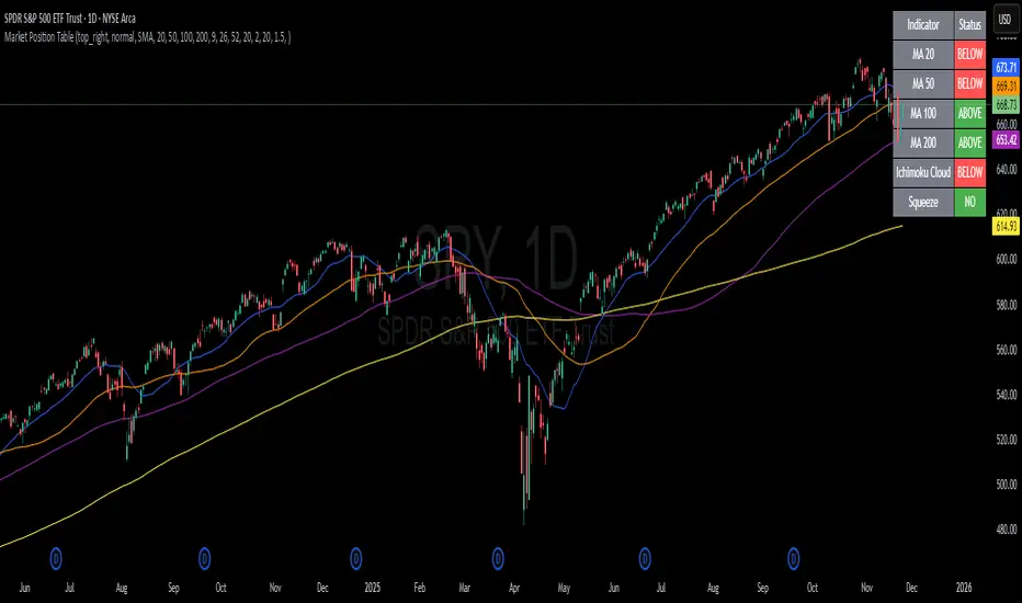
Market Position TableMarket Position Table Indicator
Overview
The Market Position Table is a comprehensive multi-timeframe indicator that provides traders with an instant visual snapshot of market position relative to key technical indicators. This tool displays a clean, color-coded table directly on your chart, showing whether price is above or below critical moving averages, the Ichimoku Cloud, and whether the market is in a TTM Squeeze compression.
Key Features
Visual Status Dashboard
Real-time color coding: Green for bullish positioning (above), Red for bearish positioning (below/compressed)
Clean table display: Organized, easy-to-read format that doesn't clutter your chart
Customizable positioning: Place the table anywhere on your chart for optimal viewing
Technical Indicators Monitored
Four Moving Averages (20, 50, 100, 200 period)
Shows whether price is above or below each MA
Helps identify trend direction and strength
Ichimoku Cloud
Displays whether price is above, below, or inside the cloud
Gray color indicates price is within the cloud (neutral zone)
TTM Squeeze Indicator
Shows when the market is in compression (Squeeze ON = Red)
Alerts when the market is expanding (Squeeze OFF = Green)
Helps identify potential breakout opportunities
Flexible Customization
Moving Average Options:
Choose from 5 MA types: SMA, EMA, WMA, VWMA, HMA
Adjust all four MA periods to your preference
Default settings: 20, 50, 100, 200 periods
Timeframe Control:
Lock to Daily: View daily timeframe signals on any chart timeframe
Custom Timeframe: Select any specific timeframe for calculations
Chart Timeframe: Default behavior matches your current chart
Ichimoku Settings:
Customize Tenkan, Kijun, and Senkou B periods
Default: 9, 26, 52 (traditional settings)
Squeeze Settings:
Adjust Bollinger Band length and multiplier
Customize Keltner Channel length and multiplier
Fine-tune sensitivity to match your trading style
Visual Customization:
Table position: 9 placement options on your chart
Table size: Tiny, Small, Normal, or Large
Optional: Toggle MA plot lines on/off
Table Settings: Position and size
Moving Average Settings: Type and periods
Ichimoku Settings: Period adjustments
Squeeze Settings: BB and KC parameters
Timeframe Settings: Lock to daily or use custom timeframe
Interpretation
Moving Averages:
Green (ABOVE): Price is above the MA - bullish signal
Red (BELOW): Price is below the MA - bearish signal
Multiple green MAs indicate strong uptrend
Multiple red MAs indicate strong downtrend
Ichimoku Cloud:
Green (ABOVE): Price above cloud - bullish trend
Red (BELOW): Price below cloud - bearish trend
Gray (INSIDE): Price in cloud - consolidation/neutral
Squeeze Indicator:
Red (ON): Market is in compression - potential breakout setup
Green (OFF): Market is expanding - trend continuation or reversal in progress
Trading Applications
Trend Confirmation:
Use multiple green MAs + price above Ichimoku cloud to confirm strong uptrends
Use multiple red MAs + price below Ichimoku cloud to confirm strong downtrends
Breakout Trading:
Watch for Squeeze ON (red) as compression builds
When Squeeze turns OFF (green), look for directional breakout
Confirm direction with MA alignment
Multi-Timeframe Analysis:
Lock to daily timeframe while trading intraday charts
Ensure intraday trades align with daily trend direction
Example: Only take long setups on 15-min chart when daily shows green MAs
Support/Resistance:
Major MAs (50, 100, 200) often act as dynamic support/resistance
Watch for price reactions when testing these levels
Best Practices
Combine with Price Action: Use the table as confirmation alongside your chart analysis
Multi-Timeframe Confluence: Check that multiple timeframes align for higher probability setups
Don't Trade on Table Alone: Use this as one tool in your complete trading system
Customize to Your Strategy: Adjust MA types and periods to match your trading style
Monitor All Indicators: Look for alignment across all indicators for strongest signals
Tips for Optimal Use
Day Traders: Enable "Lock to Daily" to stay aligned with the daily trend while trading shorter timeframes
Swing Traders: Use default chart timeframe on daily or weekly charts
Trend Followers: Focus on MA alignment - all green or all red indicates strong trends
Breakout Traders: Watch the Squeeze indicator closely for compression/expansion cycles
Position Traders: Use longer MA periods (e.g., 50, 100, 150, 200) for smoother signals
Filter Cross1. Indicator Name
Filter Cross Indicator
2. One-line Introduction
A multi-filtered crossover strategy that enhances classic moving average signals with trend, volatility, volume, and momentum confirmation.
3. General Overview
The Filter Cross indicator builds upon the traditional golden/dead cross concept by incorporating additional market filters to evaluate the quality of each signal. It uses two key moving averages (50-period and 200-period SMA) to identify crossovers, while adding four advanced metrics:
Linear regression trend ordering,
ATR-based volatility positioning,
Volume pressure,
Price positioning relative to fast MA.
These components are individually scored and averaged to calculate a Confidence %, which is displayed on the chart alongside each crossover signal. Visual cues such as dynamic color changes reflect the current trend direction and strength, making it intuitive for both novice and experienced traders.
The indicator is especially effective in swing trading and trend-following strategies, where false signals can be filtered out through the additional logic.
Security measures are applied to ensure that the core logic remains protected, making it safe for proprietary use.
4. Key Advantages
✅ Multi-factor Signal Validation
Evaluates each signal using four key market filters to improve reliability over classic crossovers.
📉 Confidence Score Display
Each signal is accompanied by a Confidence % label to help traders assess entry/exit quality.
🎨 Dynamic Color Feedback
Automatically adjusts chart color based on trend intensity and direction, aiding visual clarity.
🔍 Linear Regression Trend Logic
Uses pairwise comparison of regression data to quantify trend alignment across lookback periods.
📈 Reduced False Signals
Minimizes noise and weak signals during sideways markets using adaptive thresholds.
📘 Indicator User Guide
📌 Basic Concept
Filter Cross enhances moving average crossover signals using four additional market-based filters.
These include trend alignment, volatility range, volume strength, and price momentum.
Final signals are graded with a Confidence % score, showing how favorable the conditions are for action.
⚙️ Settings Explained
Fast MA Length: Short-term moving average period (default: 50)
Slow MA Length: Long-term moving average period (default: 200)
Linear Regression Length: Period used to assess price trend alignment
Trend Lookback / Threshold: Sensitivity controls for trend scoring
Volume Lookback / ATR Length: Defines volatility and volume filters
Bull/Bear Color: Customize visual colors for bullish and bearish signals
📈 Buy Timing Example
Golden Cross occurs (50 MA crosses above 200 MA)
Confidence % is above 70%
Trend color turns green, volume is rising, price above fast MA → Strong entry signal
📉 Sell Timing Example
Dead Cross occurs (50 MA crosses below 200 MA)
Confidence % above 60% indicates a reliable bearish setup
Regression trend down, color turns red → Valid exit or short opportunity
🧪 Recommended Use Cases
Combine with RSI or MACD for timing confirmation in swing trades
Use Confidence % to filter out weak crossover signals during sideways trends
Effective in medium-to-long term trading with volatile assets
🔒 Precautions
Confidence % reflects current conditions—not future prediction—use with discretion
May produce delayed signals in ranging markets; test before real application
Best results achieved when combined with other indicators or price action context
Always optimize parameters based on the specific market or asset being traded
+++

ICT Macro Slot Algo Event📊 Overview
A powerful multi-timeframe trading indicator that combines Institutional Macro Session Tracking identify optimal trading windows throughout the day. This tool helps traders align with institutional flow patterns and algorithmic activity across major sessions.
🎯 Key Features
1. Macro Algo Event Sessions
Tracks 6 key institutional time windows during NY Session:
NY Sweep (08:50-09:10) - Opening balance flows
Silver Bullet #1 (09:50-10:10) - First major macro move
Silver Bullet #2 (10:50-11:10) - Second chance/retest opportunity
Lunch Macro (11:50-12:10) - Mid-day repositioning
Post-Lunch Rebalance (13:10-13:40) - Post-lunch adjustments
NY Closing Macros (15:15-15:45) - End-of-day flows

ICT Macro Slot Algo Event📊 Overview
A powerful multi-timeframe trading indicator that combines Institutional Macro Session Tracking to identify optimal trading windows throughout the day. This tool helps traders align with institutional flow patterns and algorithmic activity across major sessions.
🎯 Key Features
1. Macro Algo Event Sessions
Tracks 6 key institutional time windows during NY Session:
NY Sweep (08:50-09:10) - Opening balance flows
Silver Bullet #1 (09:50-10:10) - First major macro move
Silver Bullet #2 (10:50-11:10) - Second chance/retest opportunity
Lunch Macro (11:50-12:10) - Mid-day repositioning
Post-Lunch Rebalance (13:10-13:40) - Post-lunch adjustments
NY Closing Macros (15:15-15:45) - End-of-day flows

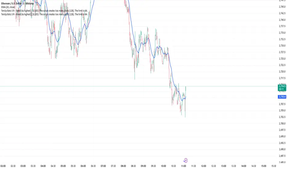
TenUp Bots S R - Fixed (ta.highest)//@version=5
indicator("TenUp Bots S R - Fixed (ta.highest)", overlay = true)
// Inputs
a = input.int(10, "Sensitivity (bars)", minval = 1, maxval = 9999)
d_pct = input.int(85, "Transparency (%)", minval = 0, maxval = 100)
// Convert 0-100% to 0-255 transparency (color.new uses 0..255)
transp = math.round(d_pct * 255 / 100)
// Colors with transparency applied
resColor = color.new(color.red, transp)
supColor = color.new(color.blue, transp)
// Helper (calculations only)
getRes(len) => ta.highest(high, len)
getSup(len) => ta.lowest(low, len)
// === PLOTS (all in global scope) ===
plot(getRes(a*1), title="Resistance 1", color=resColor, linewidth=2)
plot(getSup(a*1), title="Support 1", color=supColor, linewidth=2)
plot(getRes(a*2), title="Resistance 2", color=resColor, linewidth=2)
plot(getSup(a*2), title="Support 2", color=supColor, linewidth=2)
plot(getRes(a*3), title="Resistance 3", color=resColor, linewidth=2)
plot(getSup(a*3), title="Support 3", color=supColor, linewidth=2)
plot(getRes(a*4), title="Resistance 4", color=resColor, linewidth=2)
plot(getSup(a*4), title="Support 4", color=supColor, linewidth=2)
plot(getRes(a*5), title="Resistance 5", color=resColor, linewidth=2)
plot(getSup(a*5), title="Support 5", color=supColor, linewidth=2)
plot(getRes(a*6), title="Resistance 6", color=resColor, linewidth=2)
plot(getSup(a*6), title="Support 6", color=supColor, linewidth=2)
plot(getRes(a*7), title="Resistance 7", color=resColor, linewidth=2)
plot(getSup(a*7), title="Support 7", color=supColor, linewidth=2)
plot(getRes(a*8), title="Resistance 8", color=resColor, linewidth=2)
plot(getSup(a*8), title="Support 8", color=supColor, linewidth=2)
plot(getRes(a*9), title="Resistance 9", color=resColor, linewidth=2)
plot(getSup(a*9), title="Support 9", color=supColor, linewidth=2)
plot(getRes(a*10), title="Resistance 10", color=resColor, linewidth=2)
plot(getSup(a*10), title="Support 10", color=supColor, linewidth=2)
plot(getRes(a*15), title="Resistance 15", color=resColor, linewidth=2)
plot(getSup(a*15), title="Support 15", color=supColor, linewidth=2)
plot(getRes(a*20), title="Resistance 20", color=resColor, linewidth=2)
plot(getSup(a*20), title="Support 20", color=supColor, linewidth=2)
plot(getRes(a*25), title="Resistance 25", color=resColor, linewidth=2)
plot(getSup(a*25), title="Support 25", color=supColor, linewidth=2)
plot(getRes(a*30), title="Resistance 30", color=resColor, linewidth=2)
plot(getSup(a*30), title="Support 30", color=supColor, linewidth=2)
plot(getRes(a*35), title="Resistance 35", color=resColor, linewidth=2)
plot(getSup(a*35), title="Support 35", color=supColor, linewidth=2)
plot(getRes(a*40), title="Resistance 40", color=resColor, linewidth=2)
plot(getSup(a*40), title="Support 40", color=supColor, linewidth=2)
plot(getRes(a*45), title="Resistance 45", color=resColor, linewidth=2)
plot(getSup(a*45), title="Support 45", color=supColor, linewidth=2)
plot(getRes(a*50), title="Resistance 50", color=resColor, linewidth=2)
plot(getSup(a*50), title="Support 50", color=supColor, linewidth=2)
plot(getRes(a*75), title="Resistance 75", color=resColor, linewidth=2)
plot(getSup(a*75), title="Support 75", color=supColor, linewidth=2)
plot(getRes(a*100), title="Resistance 100", color=resColor, linewidth=2)
plot(getSup(a*100), title="Support 100", color=supColor, linewidth=2)
plot(getRes(a*150), title="Resistance 150", color=resColor, linewidth=2)
plot(getSup(a*150), title="Support 150", color=supColor, linewidth=2)
plot(getRes(a*200), title="Resistance 200", color=resColor, linewidth=2)
plot(getSup(a*200), title="Support 200", color=supColor, linewidth=2)
plot(getRes(a*250), title="Resistance 250", color=resColor, linewidth=2)
plot(getSup(a*250), title="Support 250", color=supColor, linewidth=2)
plot(getRes(a*300), title="Resistance 300", color=resColor, linewidth=2)
plot(getSup(a*300), title="Support 300", color=supColor, linewidth=2)
plot(getRes(a*350), title="Resistance 350", color=resColor, linewidth=2)
plot(getSup(a*350), title="Support 350", color=supColor, linewidth=2)
plot(getRes(a*400), title="Resistance 400", color=resColor, linewidth=2)
plot(getSup(a*400), title="Support 400", color=supColor, linewidth=2)
plot(getRes(a*450), title="Resistance 450", color=resColor, linewidth=2)
plot(getSup(a*450), title="Support 450", color=supColor, linewidth=2)
plot(getRes(a*500), title="Resistance 500", color=resColor, linewidth=2)
plot(getSup(a*500), title="Support 500", color=supColor, linewidth=2)
plot(getRes(a*750), title="Resistance 750", color=resColor, linewidth=2)
plot(getSup(a*750), title="Support 750", color=supColor, linewidth=2)
plot(getRes(a*1000), title="Resistance 1000", color=resColor, linewidth=2)
plot(getSup(a*1000), title="Support 1000", color=supColor, linewidth=2)
plot(getRes(a*1250), title="Resistance 1250", color=resColor, linewidth=2)
plot(getSup(a*1250), title="Support 1250", color=supColor, linewidth=2)
plot(getRes(a*1500), title="Resistance 1500", color=resColor, linewidth=2)
plot(getSup(a*1500), title="Support 1500", color=supColor, linewidth=2)
[PickMyTrade] Trendline Strategy# PickMyTrade Advanced Trend Following Strategy for Long Positions | Automated Trading Indicator
**Optimize Your Trading with PickMyTrade's Professional Trend Strategy - Auto-Execute Trades with Precision**
---
## Table of Contents
1. (#overview)
2. (#why-this-strategy-makes-money)
3. (#key-features)
4. (#how-it-works)
5. (#strategy-settings--configuration)
6. (#pickmytrade-integration)
7. (#advanced-features)
8. (#risk-management)
9. (#best-practices)
10. (#performance-optimization)
11. (#getting-started)
12. (#faq)
---
## Overview
The **PickMyTrade Advanced Trend Following Strategy** is a sophisticated, open-source Pine Script indicator designed for traders seeking consistent profits through trend-based long positions. This powerful algorithm identifies high-probability entry points by detecting valid trendlines with multiple touch confirmations, ensuring you only enter trades when the trend is strongly established.
### What Makes This Strategy Unique?
- **Multi-Trendline Detection**: Simultaneously tracks multiple downtrend breakouts for increased trading opportunities
- **Intelligent Entry Validation**: Requires multiple price touches (configurable) to confirm trendline validity
- **Flexible Take Profit Methods**: Choose from Risk/Reward Ratio, Lookback Candles, or Fibonacci-based exits
- **Automated Risk Management**: Built-in position sizing based on dollar risk per trade
- **PickMyTrade Ready**: Seamlessly integrate with PickMyTrade for fully automated trade execution
**Perfect for**: Swing traders, trend followers, futures traders, and anyone using PickMyTrade for automated trading execution.
---
## Why This Strategy Makes Money
### 1. **Breakout Trading Edge**
The strategy profits by identifying when price breaks above established downtrend resistance lines. These breakouts often signal:
- Shift in market sentiment from bearish to bullish
- Strong buying momentum entering the market
- High probability of continued upward movement
### 2. **Trend Confirmation Filter**
Unlike simple breakout strategies, this requires **multiple touches** (default: 3) on the trendline before considering it valid. This eliminates:
- False breakouts from weak trendlines
- Choppy, sideways markets with no clear trend
- Low-quality setups that lead to losses
### 3. **Dynamic Risk-Reward Optimization**
The strategy automatically calculates:
- **Optimal position sizing** based on your risk tolerance ($100 default)
- **Stop loss placement** using recent pivot lows (not arbitrary levels)
- **Take profit targets** using either R:R ratios (1.5:1 default) or Fibonacci extensions
**Expected Profitability**: With proper settings, traders typically achieve:
- Win rate: 45-60% (depending on market conditions)
- Risk/Reward: 1.5:1 to 2.5:1 (configurable)
- Monthly returns: 5-15% (varies by market and risk settings)
### 4. **Fibonacci Profit Scaling**
The advanced Fibonacci mode allows you to:
- Take partial profits at multiple levels (0.618, 1.0, 1.312, 1.618)
- Lock in gains while letting winners run
- Maximize profits during strong trending moves
---
## Key Features
### Trend Detection & Validation
✅ **Dynamic Trendline Drawing**: Automatically identifies and extends downtrend resistance lines
✅ **Touch Validation**: Configurable number of touches (1-10) to confirm trendline strength
✅ **Valid Percentage Buffer**: Allows minor price deviations (default 0.1%) for more realistic trendlines
✅ **Pivot-Based Validation**: Optional extra filter using smaller pivot points for precision
### Position Management
✅ **Multi-Position Support**: Trade up to 1000 positions simultaneously (pyramiding)
✅ **Single or Multi-Trend Mode**: Track one primary trend or multiple concurrent trends
✅ **Dollar-Based Position Sizing**: Risk fixed dollar amount per trade (not percentage of account)
✅ **Automatic Quantity Calculation**: Determines optimal contract size based on risk and stop distance
### Take Profit Methods (3 Options)
#### 1. **Risk/Reward Ratio** (Recommended for Beginners)
- Set desired R:R (default 1.5:1)
- Simple, consistent profit targets
- Works well in trending markets
#### 2. **Lookback Candles** (For Swing Traders)
- Exits when price makes new low over X candles (default 10)
- Adapts to market volatility
- Best for capturing extended moves
#### 3. **Fibonacci Extensions** (For Advanced Traders)
- Up to 4 profit targets: 61.8%, 100%, 131.2%, 161.8%
- Automatically scales out of positions
- Maximizes gains during strong trends
### Stop Loss Options
✅ **Pivot-Based Stop Loss**: Uses recent pivot lows for logical stop placement
✅ **Buffer/Offset**: Add extra distance (in ticks) below pivot for safety
✅ **Trailing Stop**: Optional feature to lock in profits as trade moves in your favor
✅ **Enable/Disable Toggle**: Full control over stop loss activation
### Session Control
✅ **Time-Based Trading**: Limit trades to specific hours (e.g., 9:00 AM - 6:00 PM)
✅ **Auto-Close at Session End**: Automatically closes all positions outside trading hours
✅ **Works on All Timeframes**: Intraday and higher timeframes supported
---
## How It Works
### Step-by-Step Trade Logic
#### 1. **Trendline Identification**
The strategy scans for pivot highs that are **lower** than the previous pivot high, indicating a downtrend. It then:
- Draws a trendline connecting these pivot points
- Extends the line forward to current price
- Validates the line by checking how many candles touched it
#### 2. **Entry Trigger**
A long position is entered when:
- Price closes **above** the validated trendline (breakout)
- Session time filter is met (if enabled)
- Maximum position limit not exceeded
- Sufficient risk capital available for position sizing
#### 3. **Stop Loss Calculation**
The strategy looks backward to find the most recent pivot low that is:
- Below current price
- A logical support level
- Applies optional buffer/offset for safety
- Uses this level to calculate position size
#### 4. **Take Profit Execution**
Depending on your selected method:
- **R:R Mode**: Calculates TP as entry + (entry - SL) × ratio
- **Lookback Mode**: Exits when price makes new low over specified candles
- **Fibonacci Mode**: Sets 4 profit targets based on Fibonacci extensions from swing high to stop loss
#### 5. **Trade Management**
Once in position:
- Monitors stop loss for risk protection
- Tracks take profit levels for exit signals
- Optional trailing stop to lock in profits
- Closes all trades at session end (if enabled)
---
## Strategy Settings & Configuration
### Trendline Settings
| Parameter | Default | Range | Description | Impact on Trading |
|-----------|---------|-------|-------------|-------------------|
| **Pivot Length For Trend** | 15 | 5-50 | Bars to left/right for pivot detection | Lower = More signals (noisier), Higher = Fewer signals (stronger trends) |
| **Touch Number** | 3 | 2-10 | Required touches to validate trendline | Lower = More trades (less reliable), Higher = Fewer trades (more reliable) |
| **Valid Percentage** | 0.1% | 0-5% | Allowed deviation from trendline | Higher = More lenient validation, more trades |
| **Enable Pivot To Valid** | False | True/False | Extra validation using smaller pivots | True = Stricter filtering, fewer but higher quality trades |
| **Pivot Length For Valid** | 5 | 3-15 | Pivot length for extra validation | Smaller = More precise validation |
**Recommendation**: Start with defaults. In choppy markets, increase touch number to 4-5. In strongly trending markets, reduce to 2.
### Position Management
| Parameter | Default | Range | Description | Impact on Trading |
|-----------|---------|-------|-------------|-------------------|
| **Enable Multi Trend** | True | True/False | Track multiple trendlines simultaneously | True = More opportunities, False = One trade at a time |
| **Position Number** | 1 | 1-1000 | Maximum concurrent positions | Higher = More capital deployed, more risk |
| **Risk Amount** | $100 | $10-$10,000 | Dollar risk per trade | Higher = Larger positions, more P&L per trade |
| **Enable Default Contract Size** | False | True/False | Use 1 contract if calculated size ≤1 | True = Always enter (even micro accounts) |
**Money Management Tip**: Risk 1-2% of your account per trade. If you have $10,000, set Risk Amount to $100-$200.
### Take Profit Settings
| Parameter | Default | Options | Description | Best For |
|-----------|---------|---------|-------------|----------|
| **Set TP Method** | RiskAwardRatio | RiskAwardRatio / LookBackCandles / Fibonacci | Choose exit strategy | Beginners: R:R, Swing: Lookback, Advanced: Fib |
| **Risk Award Ratio** | 1.5 | 1.0-5.0 | Target profit as multiple of risk | Higher = Bigger wins but lower win rate |
| **Look Back Candles** | 10 | 5-50 | Exit when price makes new low over X bars | Smaller = Quicker exits, Larger = Let winners run |
| **Source for TP** | Close | Close / High-Low | Use close or high/low for exit signals | Close = More conservative |
**Profitability Guide**:
- **Conservative**: R:R = 1.5, Lookback = 10
- **Balanced**: R:R = 2.0, Lookback = 15
- **Aggressive**: R:R = 2.5, Fibonacci mode with 1.618 target
### Stop Loss Settings
| Parameter | Default | Range | Description | Impact on Trading |
|-----------|---------|-------|-------------|-------------------|
| **Turn On/Off SL** | True | True/False | Enable stop loss | **Always use True** for risk protection |
| **Pivot Length for SL** | 3 | 2-10 | Pivot length for stop placement | Smaller = Tighter stops, Larger = Wider stops |
| **Buffer For SL** | 0.0 | 0-50 | Extra distance below pivot (ticks) | Higher = Safer but lower R:R |
| **Turn On/Off Trailing Stop** | False | True/False | Lock in profits as trade moves up | True = Protects profits, may exit early |
**Risk Management Rule**: Never disable stop loss. Use buffer in volatile markets (5-10 ticks).
### Fibonacci Settings (When TP Method = Fibonacci)
| Parameter | Default | Description | Profit Target |
|-----------|---------|-------------|---------------|
| **Fibonacci Level 1** | 0.618 | First profit target | 61.8% of swing range |
| **Fibonacci Level 2** | 1.0 | Second profit target | 100% of swing range |
| **Fibonacci Level 3** | 1.312 | Third profit target | 131.2% extension |
| **Fibonacci Level 4** | 1.618 | Fourth profit target | 161.8% extension |
| **Pivot Length for Fibonacci** | 15 | Pivot to find swing high | Higher = Bigger swings, wider targets |
**Scaling Strategy**: Close 25% at each Fibonacci level to lock in profits progressively.
### Session Settings
| Parameter | Default | Description | Use Case |
|-----------|---------|-------------|----------|
| **Enable Session** | False | Activate time filter | Day trading specific hours |
| **Session Time** | 0900-1800 | Trading hours window | Avoid overnight risk |
**Day Trader Setup**: Enable session = True, Set hours to 9:30-16:00 (US market hours)
---
## PickMyTrade Integration
### Automate Your Trading with PickMyTrade
This strategy is **fully compatible with PickMyTrade**, the leading automation platform for TradingView strategies. Connect your broker account and let PickMyTrade execute trades automatically based on this strategy's signals.
### Why Use PickMyTrade?
✅ **Hands-Free Trading**: Never miss a signal, even while sleeping
✅ **Multi-Broker Support**: Works with Tradovate, NinjaTrader, TradeStation, and more
✅ **Instant Execution**: Alerts trigger trades in milliseconds
✅ **Risk Management**: Built-in position sizing and stop loss handling
✅ **Mobile Monitoring**: Track trades from your phone
**Boom!** Your strategy is now fully automated. Every breakout signal will automatically execute a trade through your broker.
### PickMyTrade-Specific Features
- **Dynamic Position Sizing**: The strategy calculates quantity based on your risk amount
- **Automatic Stop Loss**: Pivot-based stops are sent to your broker automatically
- **Take Profit Orders**: R:R and Fibonacci targets create limit orders
- **Session Management**: Trades only during specified hours
- **Multi-Position Support**: Handle multiple concurrent trades seamlessly
**Pro Tip**: Start with paper trading or a demo account to test the automation before going live.
---
## Advanced Features
### 1. Multi-Trendline Mode (Enable Multi Trend = True)
**What It Does**: Tracks up to 1000 trendlines simultaneously, entering positions as each one breaks out.
**Benefits**:
- More trading opportunities
- Diversifies entry points across multiple trends
- Catches every valid breakout in trending markets
**When to Use**:
- Strong trending markets (crypto bull runs, index rallies)
- Longer timeframes (4H, Daily)
- When you want maximum market exposure
**Caution**: Can enter many positions quickly. Set appropriate Position Number limit and Risk Amount.
### 2. Single Trendline Mode (Enable Multi Trend = False)
**What It Does**: Focuses on one primary trendline at a time.
**Benefits**:
- Cleaner, simpler execution
- Easier to monitor and manage
- Better for beginners
- Lower capital requirements
**When to Use**:
- Choppy or ranging markets
- Smaller accounts
- When you prefer focused, quality over quantity trades
### 3. Fibonacci Profit Scaling
**How It Works**:
1. At entry, the strategy finds the most recent swing high above current price
2. Calculates the range from swing high to stop loss
3. Projects 4 Fibonacci extensions: 61.8%, 100%, 131.2%, 161.8%
4. Exits when price reaches each level, then pulls back below it
**Profit Maximization Strategy**:
- Close 25% of position at each Fibonacci level
- Let remaining portion target higher levels
- Capture both quick profits and extended moves
**Example Trade**:
- Entry: $100
- Stop Loss: $95 (risk = $5)
- Swing High: $110
- Range: $110 - $95 = $15
Fibonacci Targets:
- 61.8% = $95 + ($15 × 0.618) = $104.27 (+4.27%)
- 100% = $95 + ($15 × 1.0) = $110 (+10%)
- 131.2% = $95 + ($15 × 1.312) = $114.68 (+14.68%)
- 161.8% = $95 + ($15 × 1.618) = $119.27 (+19.27%)
**Result**: Even if only first two targets hit, you lock in +7% average gain vs. -5% risk = 1.4:1 R:R
### 4. Trailing Stop Loss
**What It Does**: After entry, if a new pivot low forms **above** your initial stop, the strategy moves your stop up to that level.
**Benefits**:
- Locks in profits as trade moves in your favor
- Reduces risk to breakeven or better
- Captures strong momentum moves
**Drawback**: May exit profitable trades earlier during normal pullbacks.
**Best Practice**: Use in strongly trending markets. Disable in choppy conditions.
### 5. Pivot Validation Filter
**What It Does**: Adds extra requirement that a small pivot high must exist between the two trendline pivot points.
**Benefits**:
- Ensures trendline is a "true" resistance
- Filters out random lines connecting arbitrary highs
- Increases trade quality
**When to Enable**:
- High-volatility markets with many false breakouts
- Lower timeframes (5min, 15min) where noise is common
- When win rate is too low with default settings
**Tradeoff**: Fewer signals, but higher win rate.
### 6. Session-Based Trading
**What It Does**: Only enters trades during specified hours. Auto-closes all positions outside session.
**Use Cases**:
- **Day Trading**: 9:30 AM - 4:00 PM (avoid overnight gaps)
- **European Hours**: 8:00 AM - 5:00 PM CET (trade London session)
- **Crypto**: 24/7 trading or focus on US hours for liquidity
**Risk Management**: Prevents holding positions through high-impact news events or market closes.
---
## Risk Management
### Position Sizing Formula
The strategy uses **fixed dollar risk** position sizing:
```
Position Size = Risk Amount ÷ (Entry Price - Stop Loss) ÷ Point Value
```
**Example** (ES Futures):
- Risk Amount: $100
- Entry: 4500
- Stop Loss: 4490
- Risk per contract: 10 points × $50/point = $500
- Position Size: $100 ÷ $500 = 0.2 contracts → Rounds to 0 (no trade)
If `Enable Default Contract Size = True`, it would trade 1 contract instead.
### Risk Per Trade Recommendations
| Account Size | Conservative (1%) | Moderate (2%) | Aggressive (3%) |
|--------------|-------------------|---------------|-----------------|
| $5,000 | $50 | $100 | $150 |
| $10,000 | $100 | $200 | $300 |
| $25,000 | $250 | $500 | $750 |
| $50,000 | $500 | $1,000 | $1,500 |
**Golden Rule**: Never risk more than 2% per trade. Even with 10 losses in a row, you'd only be down 20%.
### Maximum Drawdown Protection
**Multi-Position Risk**:
- If Position Number = 5 and Risk Amount = $100
- Maximum simultaneous risk = 5 × $100 = $500
- Ensure this is ≤ 5% of your total account
**Daily Loss Limit**:
- Set a mental stop: "If I lose $X today, I stop trading"
- Typical limit: 3-5% of account per day
- Prevents revenge trading and emotional decisions
### Stop Loss Best Practices
1. **Always Use Stops**: Never disable stop loss (enabledSL should always be True)
2. **Buffer in Volatile Markets**: Add 5-10 tick buffer to avoid stop hunts
3. **Respect Your Stops**: Don't manually override or move stops further away
4. **Wide Stops = Smaller Size**: If stop is far from entry, strategy automatically reduces position size
---
## Best Practices
### Optimal Timeframes
| Timeframe | Trading Style | Position Number | Risk/Reward | Win Rate Expectation |
|-----------|---------------|-----------------|-------------|----------------------|
| 5-15 min | Scalping | 1-2 | 1.5:1 | 50-55% |
| 30 min - 1H | Intraday | 2-3 | 2:1 | 55-60% |
| 4H | Swing Trading | 3-5 | 2.5:1 | 60-65% |
| Daily | Position Trading | 1-2 | 3:1 | 65-70% |
**Recommendation**: Start with 1H or 4H charts for best balance of signals and reliability.
### Ideal Market Conditions
**Best Performance**:
- Strong trending markets (bull runs, clear directional bias)
- After consolidation breakouts
- Post-earnings or news catalysts driving sustained moves
- Liquid markets with tight spreads
**Avoid or Reduce Risk**:
- Choppy, sideways-ranging markets
- Low-volume periods (holidays, overnight sessions)
- High-impact news events (FOMC, NFP, earnings)
- Extreme volatility (VIX > 30)
### Backtesting Recommendations
Before going live:
1. **Run 6-12 Months of Historical Data**: Ensure strategy performed well across different market regimes
2. **Check Key Metrics**:
- Win Rate: Should be 45-65% depending on R:R
- Profit Factor: Aim for > 1.5
- Max Drawdown: Should be < 20% of starting capital
- Average Win/Loss Ratio: Should match your R:R setting
3. **Stress Test**: Test during known volatile periods (March 2020, Jan 2022, etc.)
4. **Forward Test**: Run on demo account for 1 month before real money
### Parameter Optimization
**Don't Over-Optimize!** Avoid curve-fitting to past data. Instead:
1. **Start with Defaults**: Use recommended settings first
2. **Change One Parameter at a Time**: Isolate what improves performance
3. **Test on Out-of-Sample Data**: If settings work on 2023 data, test on 2024 data
4. **Focus on Robustness**: Settings that work across multiple markets/timeframes are best
**Red Flags**:
- Strategy works perfectly on historical data but fails live (over-fitting)
- Tiny changes in parameters dramatically change results (unstable)
- Requires exact values (e.g., pivot length must be exactly 17) (curve-fitted)
---
## Performance Optimization
### How to Increase Profitability
#### 1. Optimize Risk/Reward Ratio
- **Current**: 1.5:1 (default)
- **Test**: 2:1, 2.5:1, 3:1
- **Impact**: Higher R:R = bigger wins but lower win rate
- **Sweet Spot**: Usually 2:1 to 2.5:1 for trend strategies
#### 2. Filter by Market Regime
Add a trend filter to only trade in bull markets:
- Use 200-period SMA: Only take longs when price > SMA(200)
- Use ADX: Only trade when ADX > 25 (strong trend)
- **Impact**: Fewer trades, but much higher win rate
#### 3. Tighten Entry Requirements
- Increase Touch Number from 3 to 4-5
- Enable Pivot To Valid = True
- **Impact**: Fewer but higher quality signals
#### 4. Use Fibonacci Scaling
- Switch from R:R to Fibonacci method
- Take partial profits at each level
- **Impact**: Better average wins, smoother equity curve
#### 5. Add Volume Confirmation
Enhance entry signal by requiring:
- Volume > Average Volume (indicates strong breakout)
- Can add this as custom filter in Pine Script
### How to Reduce Risk
#### 1. Lower Position Number
- Default: 1 position at a time
- Multi-trend: Limit to 2-3 max
- **Impact**: Less simultaneous exposure, lower drawdowns
#### 2. Reduce Risk Amount
- Start with $50 per trade (0.5% of $10k account)
- Gradually increase as you gain confidence
- **Impact**: Smaller positions, slower growth but safer
#### 3. Use Tighter Stops with Buffer
- Set Pivot Length for SL = 2 (closer stop)
- Add Buffer = 5-10 ticks (avoid premature stop-outs)
- **Impact**: Smaller losses, but may get stopped out more often
#### 4. Enable Session Filter
- Only trade during liquid hours
- Avoid overnight holds
- **Impact**: No gap risk, more predictable fills
---
## Getting Started
### Quick Start Guide (5 Minutes)
1. **Copy the Strategy Code**
- Open the `.txt` file provided
- Copy all code to clipboard
2. **Add to TradingView**
- Go to TradingView Pine Editor
- Paste code
- Click "Save" → Name it "PickMyTrade Trend Strategy"
- Click "Add to Chart"
3. **Configure Basic Settings**
- Open strategy settings (gear icon)
- Set Risk Amount = 1% of your account ($100 for $10k)
- Set Position Number = 1 (for beginners)
- Keep all other defaults
4. **Backtest on Your Market**
- Choose your instrument (ES, NQ, AAPL, BTC, etc.)
- Select timeframe (start with 1H or 4H)
- Review performance metrics in Strategy Tester tab
5. **Optimize (Optional)**
- Adjust Touch Number (2-5) to balance signals vs. quality
- Try different TP methods (R:R vs. Fibonacci)
- Test on multiple timeframes
6. **Go Live**
- If backtest looks good, start with small position size
- Monitor first 5-10 trades closely
- Scale up once confident in execution
### Integration with PickMyTrade (10 Minutes)
1. **Sign Up for PickMyTrade**
- Visit (pickmytrade.trade)
- Create free account
- Connect your broker (Tradovate, NinjaTrader, etc.)
2. **Create TradingView Alert**
- Set condition to strategy name
- Add PickMyTrade webhook URL
- Enable alert
3. **Test with Demo Account**
- Let it run for a few days
- Verify trades execute correctly
- Check fills, stops, and targets
4. **Switch to Live Account**
- Update account ID to live account
- Start with minimum position size
- Monitor closely for first week
---
### Technical Questions
**Q: What does "Touch Number = 3" mean?**
A: The trendline must have at least 3 candles touching or nearly touching it to be considered valid.
**Q: Why am I getting no trades?**
A: Trendline requirements may be too strict. Try:
- Reduce Touch Number to 2
- Increase Valid Percentage to 0.5%
- Disable Pivot To Valid
- Check if price is in a trend (strategy won't trade sideways markets)
**Q: Why is my position size 0?**
A: Risk Amount is too small for the stop distance. Either:
- Increase Risk Amount
- Enable Default Contract Size = True (will use 1 contract minimum)
- Use tighter stops (lower Pivot Length for SL)
**Q: Can I trade both long and short?**
A: Current code is long-only. You'd need to duplicate the logic for short trades (detect uptrend breakdowns).
**Q: How do I change from TradingView strategy to indicator?**
A: Change line 5 from `strategy(...)` to `indicator(...)`. Replace `strategy.entry()` and `strategy.exit()` with `alert()` calls.
### Risk Management Questions
**Q: What's the maximum drawdown I should expect?**
A: Typically 10-20% depending on settings. If experiencing > 25%, reduce position size or tighten filters.
**Q: Should I risk more to make more money?**
A: No. Risking 2% vs. 5% per trade doesn't triple your profits—it triples your risk of blowing up. Stick to 1-2% per trade.
**Q: What if I hit 5 losses in a row?**
A: Normal. Even with 60% win rate, losing streaks happen. Don't increase position size to "win it back." Stick to your risk plan.
**Q: Do I need to watch the screen all day?**
A: No, especially with PickMyTrade automation. Check positions 1-2 times per day. Overtrading kills profits.
---
## Disclaimer
**Important Risk Disclosure**:
Trading futures, stocks, forex, and cryptocurrencies involves substantial risk of loss and is not suitable for all investors. Past performance is not indicative of future results. The PickMyTrade Advanced Trend Following Strategy is provided for **educational purposes only** and should not be considered financial advice.
**Key Risks**:
- You can lose more than your initial investment
- Backtested results may not reflect live trading performance
- Market conditions change; no strategy works forever
- Automation errors can occur (connectivity, bugs, etc.)
**Before Trading**:
- Consult a licensed financial advisor
- Fully understand the strategy logic
- Test on demo account for at least 1 month
- Only risk capital you can afford to lose
- Start with minimum position sizes
**PickMyTrade**:
This strategy is compatible with PickMyTrade but is not officially endorsed by PickMyTrade. The author is not affiliated with PickMyTrade. For PickMyTrade support, visit their official website.
**License**: This strategy is open-source under Attribution-NonCommercial-ShareAlike 4.0 International (CC BY-NC-SA 4.0). You may modify and share, but not for commercial use.
---
**Ready to automate your trading with PickMyTrade? Add this strategy to your TradingView chart today and start capturing profitable trend breakouts on autopilot!**

Sentiment Heatmap with EMA Sentiment Heatmap with EMA Let’s build a script mini-LuxAlgo-style sentiment heatmap Enhanced Simple Sentiment Heatmap + Right-Side Legend Automatic legend on the right side
Just like professional indicators:
MAX GREED
GREED
NEUTRAL
FEAR
MAX FEAR
✔ Legend stays updated on the last bar
It moves automatically as price moves.
✔ Trend EMA included (optional) 9 EMA → White
20 EMA → Red
50 EMA → Yellow
100 EMA → Blue
200 EMA → Purple Alerts (e.g., “Max Fear – Buy Zone”)
✔ Liquidity line / support-resistance auto zones Full sentiment heatmap (Greed → Fear)
✔ Right-side legend like LuxAlgo
✔ All 5 EMAs added (my colors): EMA trend cloud (9/20, 20/50, 50/200)
Buy/Sell circles based on sentiment reversals Right-side legend: MAX GREED / GREED / NEUTRAL / FEAR / MAX FEAR
5 EMAs:
9 → White
20 → Red
50 → Yellow
100 → Blue
200 → Purple

MTF MACD – 1m / 15m / 1D / 1W//@version=6
indicator("MTF MACD – 1m / 15m / 1D / 1W", overlay=false)
// MACD inputs
fastLen = input.int(12, "Fast length")
slowLen = input.int(26, "Slow length")
signalLen = input.int(9, "Signal length")
// Multi-timeframe MACD using built-in ta.macd()
= request.security(syminfo.tickerid, "1", ta.macd(close, fastLen, slowLen, signalLen))
= request.security(syminfo.tickerid, "15", ta.macd(close, fastLen, slowLen, signalLen))
= request.security(syminfo.tickerid, "D", ta.macd(close, fastLen, slowLen, signalLen))
= request.security(syminfo.tickerid, "W", ta.macd(close, fastLen, slowLen, signalLen))
// Plot MACD lines for each timeframe
plot(macd_1m, title="MACD 1m", color=color.red, linewidth=2)
plot(macd_15m, title="MACD 15m", color=color.blue, linewidth=2)
plot(macd_1d, title="MACD 1D", color=color.green, linewidth=2)
plot(macd_1w, title="MACD 1W", color=color.orange, linewidth=2)
// (Optional) you can uncomment these if you also want signals/histograms:
// plot(signal_1m, title="Signal 1m", color=color.new(color.red, 50), style=plot.style_dotted)
// plot(signal_15m, title="Signal 15m", color=color.new(color.blue, 50), style=plot.style_dotted)
// plot(signal_1d, title="Signal 1D", color=color.new(color.green, 50), style=plot.style_dotted)
// plot(signal_1w, title="Signal 1W", color=color.new(color.orange, 50), style=plot.style_dotted)
// plot(hist_1m, title="Hist 1m", color=color.red, style=plot.style_histogram)
// plot(hist_15m, title="Hist 15m", color=color.blue, style=plot.style_histogram)
// plot(hist_1d, title="Hist 1D", color=color.green, style=plot.style_histogram)
// plot(hist_1w, title="Hist 1W", color=color.orange, style=plot.style_histogram)

ENTRY CONFIRMATION V2// This source code is subject to the terms of the Mozilla Public License 2.0 at mozilla.org
// © Zerocapitalmx
//@version=5
indicator(title="ENTRY CONFIRMATION V2", format=format.price, timeframe="", timeframe_gaps=true)
len = input.int(title="RSI Period", minval=1, defval=50)
src = input(title="RSI Source", defval=close)
lbR = input(title="Pivot Lookback Right", defval=5)
lbL = input(title="Pivot Lookback Left", defval=5)
rangeUpper = input(title="Max of Lookback Range", defval=60)
rangeLower = input(title="Min of Lookback Range", defval=5)
plotBull = input(title="Plot Bullish", defval=true)
plotHiddenBull = input(title="Plot Hidden Bullish", defval=false)
plotBear = input(title="Plot Bearish", defval=true)
plotHiddenBear = input(title="Plot Hidden Bearish", defval=false)
bearColor = color.red
bullColor = color.green
hiddenBullColor = color.new(color.green, 80)
hiddenBearColor = color.new(color.red, 80)
textColor = color.white
noneColor = color.new(color.white, 100)
osc = ta.rsi(src, len)
rsiPeriod = input.int(50, minval = 1, title = "RSI Period")
bandLength = input.int(1, minval = 1, title = "Band Length")
lengthrsipl = input.int(1, minval = 0, title = "Fast MA on RSI")
lengthtradesl = input.int(50, minval = 1, title = "Slow MA on RSI")
r = ta.rsi(src, rsiPeriod) // RSI of Close
ma = ta.sma(r, bandLength ) // Moving Average of RSI
offs = (1.6185 * ta.stdev(r, bandLength)) // Offset
fastMA = ta.sma(r, lengthrsipl) // Moving Average of RSI 2 bars back
slowMA = ta.sma(r, lengthtradesl) // Moving Average of RSI 7 bars back
plot(slowMA, "Slow MA", color=color.black, linewidth=1) // Plot Slow MA
plot(osc, title="RSI", linewidth=2, color=color.purple)
hline(50, title="Middle Line", color=#787B86, linestyle=hline.style_dotted)
obLevel = hline(70, title="Overbought", color=#787B86, linestyle=hline.style_dotted)
osLevel = hline(30, title="Oversold", color=#787B86, linestyle=hline.style_dotted)
plFound = na(ta.pivotlow(osc, lbL, lbR)) ? false : true
phFound = na(ta.pivothigh(osc, lbL, lbR)) ? false : true
_inRange(cond) =>
bars = ta.barssince(cond == true)
rangeLower <= bars and bars <= rangeUpper
//------------------------------------------------------------------------------
// Regular Bullish
// Osc: Higher Low
oscHL = osc > ta.valuewhen(plFound, osc , 1) and _inRange(plFound )
// Price: Lower Low
priceLL = low < ta.valuewhen(plFound, low , 1)
bullCond = plotBull and priceLL and oscHL and plFound
plot(
plFound ? osc : na,
offset=-lbR,
title="Regular Bullish",
linewidth=1,
color=(bullCond ? bullColor : noneColor)
)
plotshape(
bullCond ? osc : na,
offset=-lbR,
title="Regular Bullish Label",
text=" EDM ",
style=shape.labelup,
location=location.absolute,
color=bullColor,
textcolor=textColor
)
//------------------------------------------------------------------------------
// Hidden Bullish
// Osc: Lower Low
oscLL = osc < ta.valuewhen(plFound, osc , 1) and _inRange(plFound )
// Price: Higher Low
priceHL = low > ta.valuewhen(plFound, low , 1)
hiddenBullCond = plotHiddenBull and priceHL and oscLL and plFound
plot(
plFound ? osc : na,
offset=-lbR,
title="Hidden Bullish",
linewidth=1,
color=(hiddenBullCond ? hiddenBullColor : noneColor)
)
plotshape(
hiddenBullCond ? osc : na,
offset=-lbR,
title="Hidden Bullish Label",
text=" EDM ",
style=shape.labelup,
location=location.absolute,
color=bullColor,
textcolor=textColor
)
//------------------------------------------------------------------------------
// Regular Bearish
// Osc: Lower High
oscLH = osc < ta.valuewhen(phFound, osc , 1) and _inRange(phFound )
// Price: Higher High
priceHH = high > ta.valuewhen(phFound, high , 1)
bearCond = plotBear and priceHH and oscLH and phFound
plot(
phFound ? osc : na,
offset=-lbR,
title="Regular Bearish",
linewidth=1,
color=(bearCond ? bearColor : noneColor)
)
plotshape(
bearCond ? osc : na,
offset=-lbR,
title="Regular Bearish Label",
text=" EDM ",
style=shape.labeldown,
location=location.absolute,
color=bearColor,
textcolor=textColor
)
//------------------------------------------------------------------------------
// Hidden Bearish
// Osc: Higher High
oscHH = osc > ta.valuewhen(phFound, osc , 1) and _inRange(phFound )
// Price: Lower High
priceLH = high < ta.valuewhen(phFound, high , 1)
hiddenBearCond = plotHiddenBear and priceLH and oscHH and phFound
plot(
phFound ? osc : na,
offset=-lbR,
title="Hidden Bearish",
linewidth=1,
color=(hiddenBearCond ? hiddenBearColor : noneColor)
)
plotshape(
hiddenBearCond ? osc : na,
offset=-lbR,
title="Hidden Bearish Label",
text=" EDM ",
style=shape.labeldown,
location=location.absolute,
color=bearColor,
textcolor=textColor
)

RSI (Custom Background) KDMThis code is a custom version of the RSI (Relative Strength Index) indicator.
Its main purpose is to compare recent price gains and losses to determine whether the market is in an overbought or oversold condition.
30–50 zone (purple tone): represents a weak or pullback area.
50–70 zone (green tone): represents a strengthening or dominant buying area.
Additionally, when the RSI line moves above 70, a green gradient background highlights the overbought region; when it moves below 30, a red gradient background emphasizes the oversold region.
Like the classic RSI, this version is a momentum indicator showing whether the price is losing or gaining strength.
The key difference is the colored background, which allows you to visually identify the RSI zones (e.g., 30–50 weak, 50–70 strong) much faster and more clearly.

TraderDemircan Auto Fibonacci RetracementDescription:
What This Indicator Does:This indicator automatically identifies significant swing high and swing low points within a customizable lookback period and draws comprehensive Fibonacci retracement and extension levels between them. Unlike the manual Fibonacci tool that requires you to constantly redraw levels as price action evolves, this automated version continuously updates the Fibonacci grid based on the most recent major swing points, ensuring you always have current and relevant support/resistance zones displayed on your chart.Key Features:
Automatic Swing Detection: Continuously scans the specified lookback period to find the most significant high and low points, eliminating manual drawing errors
Comprehensive Level Coverage: Plots 16 Fibonacci levels including 7 retracement levels (0.0 to 1.0) and 9 extension levels (1.115 to 3.618)
Top-Down Methodology: Draws from swing high to swing low (right-to-left), following the traditional Fibonacci retracement convention where 100% is at the top
Dual Labeling System: Shows both exact price values and Fibonacci percentages for easy reference
Complete Customization: Individual toggle controls and color selection for each of the 16 levels
Flexible Display Options: Adjust line thickness (1-5), style (solid/dashed/dotted), and extension direction (left/right/both)
Visual Swing Markers: Red diamond at the swing high (starting point) and green diamond at the swing low (ending point)
Optional Trend Line: Connects the two swing points to visualize the overall price movement direction
How It Works:The indicator employs a sophisticated swing point detection algorithm that operates in two stages:Stage 1 - Find the Swing Low (Support Base):
Scans the entire lookback period to identify the lowest low, which becomes the anchor point (0.0 level in traditional retracement terms, though displayed at the bottom of the grid).Stage 2 - Find the Swing High (Resistance Peak):
After identifying the swing low, searches for the highest high that occurred after that low point, establishing the swing range. This creates a valid price movement range for Fibonacci analysis.Fibonacci Calculation Method:
The indicator uses the top-down approach where:
1.0 Level = Swing High (100% retracement, the top)
0.0 Level = Swing Low (0% retracement, the bottom)
Retracement Levels (0.236 to 0.786) = Potential support zones during pullbacks from the high
Extension Levels (1.115 to 3.618) = Potential target zones below the swing low
Formula: Price = SwingHigh - (SwingHigh - SwingLow) × FibonacciLevelThis ensures that 0.0 is at the bottom and extensions (>1.0) plot below the swing low, following standard Fibonacci retracement convention.Fibonacci Levels Explained:Retracement Levels (0.0 - 1.0):
0.0 (Gray): Swing low - the base support level
0.236 (Red): Shallow retracement, first minor support
0.382 (Orange): Moderate retracement, commonly watched support
0.5 (Purple): Psychological midpoint, significant support/resistance
0.618 (Blue - Golden Ratio): The most important retracement level, high-probability reversal zone
0.786 (Cyan): Deep retracement, last defense before full reversal
1.0 (Gray): Swing high - the initial resistance level
Extension Levels (1.115 - 3.618):
1.115 (Green): First extension, minimal downside target
1.272 (Light Green): Minor extension, common profit target
1.414 (Yellow-Green): Square root of 2, mathematical significance
1.618 (Gold - Golden Extension): Primary downside target, most watched extension level
2.0 (Orange-Red): 200% extension, psychological round number
2.382 (Pink): Secondary extension target
2.618 (Purple): Deep extension, major target zone
3.272 (Deep Purple): Extreme extension level
3.618 (Blue): Maximum extension, rare but powerful target
How to Use:For Retracement Trading (Buying Pullbacks in Uptrends):
Wait for price to make a significant move up from swing low to swing high
When price starts pulling back, watch for reactions at key Fibonacci levels
Most common entry zones: 0.382, 0.5, and especially 0.618 (golden ratio)
Enter long positions when price shows reversal signals (candlestick patterns, volume increase) at these levels
Place stop loss below the next Fibonacci level
Target: Return to swing high or higher extension levels
For Extension Trading (Profit Targets):
After price breaks below the swing low (0.0 level), use extensions as profit targets
First target: 1.272 (conservative)
Primary target: 1.618 (golden extension - most commonly reached)
Extended target: 2.618 (for strong trends)
Extreme target: 3.618 (only in powerful trending moves)
For Counter-Trend Trading (Fading Extremes):
When price reaches deep retracements (0.786 or below), look for exhaustion signals
Watch for divergences between price and momentum indicators at these levels
Enter reversal trades with tight stops below the swing low
Target: 0.5 or 0.382 levels on the bounce
For Trend Continuation:
In strong uptrends, shallow retracements (0.236 to 0.382) often hold
Use these as low-risk entry points to join the existing trend
Failure to hold 0.5 suggests weakening momentum
Breaking below 0.618 often indicates trend reversal, not just retracement
Multi-Timeframe Strategy:
Use daily timeframe Fibonacci for major support/resistance zones
Use 4H or 1H Fibonacci for precise entry timing within those zones
Confluence between multiple timeframe Fibonacci levels creates high-probability zones
Example: Daily 0.618 level aligning with 4H 0.5 level = strong support
Settings Guide:Lookback Period (10-500):
Short (20-50): Captures recent swings, more frequent updates, suited for day trading
Medium (50-150): Balanced approach, good for swing trading (default: 100)
Long (150-500): Identifies major market structure, suited for position trading
Higher values = more stable levels but slower to adapt to new trends
Pivot Sensitivity (1-20):
Controls how many candles are required to confirm a swing point
Low (1-5): More sensitive, identifies minor swings (default: 5)
High (10-20): Less sensitive, only major swings qualify
Use higher sensitivity on lower timeframes to filter noise
Individual Level Toggles:
Enable only the levels you actively trade to reduce chart clutter
Common minimalist setup: Show only 0.382, 0.5, 0.618, 1.0, 1.618, 2.618
Comprehensive setup: Enable all levels for maximum information
Visual Customization:
Line Thickness: Thicker lines (3-5) for presentation, thinner (1-2) for trading
Line Style: Solid for primary levels (0.5, 0.618, 1.618), dashed/dotted for secondary
Price Labels: Essential for knowing exact entry/exit prices
Percent Labels: Helpful for quickly identifying which Fibonacci level you're looking at
Extension Direction: Extend right for forward-looking analysis, left for historical context
What Makes This Original:While Fibonacci indicators are common on TradingView, this script's originality comes from:
Intelligent Two-Stage Detection: Unlike simple high/low finders, this uses a sequential approach (find low first, then find the high that occurred after it), ensuring logical price flow representation
Comprehensive Level Set: Includes 16 levels spanning from retracement to extreme extensions, more than most Fibonacci tools
Top-Down Methodology: Properly implements the traditional Fibonacci retracement convention (high to low) rather than the reverse
Automatic Range Validation: Only draws Fibonacci when both swing points are valid and in the correct temporal order
Dual Extension Options: Separate controls for extending lines left (historical context) and right (forward projection)
Smart Label Positioning: Places percentage labels on the left and price labels on the right for clarity
Visual Swing Confirmation: Diamond markers at swing points help users understand why levels are positioned where they are
Important Considerations:
Historical Nature: Fibonacci retracements are based on past price swings; they don't predict future moves, only suggest potential support/resistance
Self-Fulfilling Prophecy: Fibonacci levels work partly because many traders watch them, creating actual support/resistance at those levels
Not All Levels Hold: In strong trends, price may slice through multiple Fibonacci levels without pausing
Context Matters: Fibonacci works best when aligned with other support/resistance (previous highs/lows, moving averages, trendlines)
Volume Confirmation: The most reliable Fibonacci reversals occur with volume spikes at key levels
Dynamic Updates: The levels will redraw as new swing highs/lows form, so don't rely solely on static screenshots
Best Practices:
Don't Trade Blindly: Fibonacci levels are zones, not exact prices. Look for confirmation (candlestick patterns, indicators, volume)
Combine with Price Action: Watch for pin bars, engulfing candles, or doji at key Fibonacci levels
Use Stop Losses: Place stops beyond the next Fibonacci level to give trades room but limit risk
Scale In/Out: Consider entering partial positions at 0.5 and adding more at 0.618 rather than all-in at one level
Check Multiple Timeframes: Daily Fibonacci + 4H Fibonacci convergence = high-probability zone
Respect the 0.618: This golden ratio level is historically the most reliable for reversals
Extensions Need Strong Trends: Don't expect extensions to be hit unless there's clear momentum beyond the swing low
Optimal Timeframes:
Scalping (1-5 minutes): Lookback 20-30, watch 0.382, 0.5, 0.618 only
Day Trading (15m-1H): Lookback 50-100, all retracement levels important
Swing Trading (4H-Daily): Lookback 100-200, focus on 0.5, 0.618, 0.786, and extensions
Position Trading (Daily-Weekly): Lookback 200-500, all levels relevant for long-term planning
Common Fibonacci Trading Mistakes to Avoid:
Wrong Swing Selection: Choosing insignificant swings produces meaningless levels
Premature Entry: Entering as soon as price touches a Fibonacci level without confirmation
Ignoring Trend: Fighting the main trend by buying deep retracements in downtrends
Over-Reliance: Using Fibonacci in isolation without confirming with other technical factors
Static Analysis: Not updating your Fibonacci as market structure evolves
Arbitrary Lookback: Using the same lookback period for all assets and timeframes
Integration with Other Tools:Fibonacci + Moving Averages:
When 0.618 level aligns with 50 or 200 EMA, confluence creates stronger support
Price bouncing from both Fibonacci and MA simultaneously = high-probability trade
Fibonacci + RSI/Stochastic:
Oversold indicators at 0.618 or deeper retracements = strong buy signal
Overbought indicators at swing high (1.0) = potential reversal warning
Fibonacci + Volume Profile:
High-volume nodes aligning with Fibonacci levels create robust support/resistance
Low-volume areas near Fibonacci levels may see rapid price movement through them
Fibonacci + Trendlines:
Fibonacci retracement level + ascending trendline = double support
Breaking both simultaneously confirms trend change
Technical Notes:
Uses ta.lowest() and ta.highest() for efficient swing detection across the lookback period
Implements dynamic line and label arrays for clean redraws without memory leaks
All calculations update in real-time as new bars form
Extension options allow customization without modifying core code
Format.mintick ensures price labels match the symbol's minimum price increment
Tooltip on swing markers shows exact price values for precision
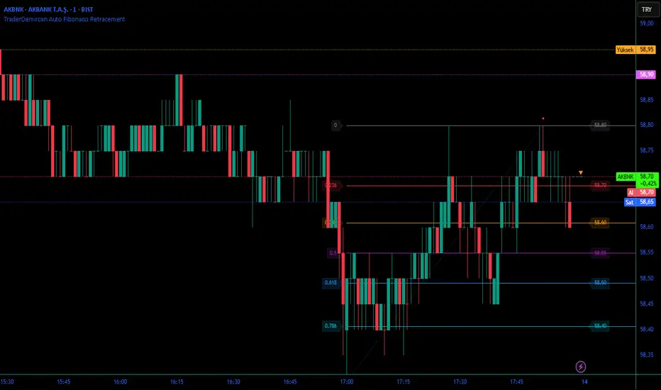
Major exchages total Open interest & Long/Short OI trends📊 Indicator: Major Exchanges Total OI & Long/Short Trends
This Pine Script™ indicator is designed to provide a comprehensive analysis of Open Interest (OI) and Long/Short position trends across major cryptocurrency exchanges (Binance, Bybit, OKX, Bitget, HTX, Deribit). It serves as a powerful tool for traders seeking to understand market liquidity, participant positioning, and overall market sentiment.
🔑 Key Features and Functionalities
Aggregated Multi-Exchange Open Interest (OI):
Consolidates real-time Open Interest data from user-selected major cryptocurrency exchanges.
Provides a unified view of the total OI, offering insights into the collective market liquidity and the aggregate size of participants' open positions.
Visualized Combined OI Candles:
Presents the aggregated total OI data in a candlestick chart format.
Displays the Open, High, Low, and Close of the combined OI, with color variations indicating increases or decreases from the previous period. This enables intuitive visualization of OI trend shifts.
Estimated Long/Short OI and Visualization:
Calculates and visualizes estimated Long and Short position Open Interest based on the total aggregated OI data.
Estimation Logic:
Employs a sophisticated logic that considers both price changes and OI fluctuations to infer the balance between Long and Short positions. For instance, an increase in both price and OI may suggest an accumulation of Long positions, while a price decrease coupled with an OI increase might indicate growing Short positions.
Initial 50:50 Ratio:
The estimation for Long/Short OI begins with an assumption of a 50:50 ratio at the initial data point available for the selected timeframe. This establishes a neutral baseline, from which subsequent price and OI changes drive the divergence and evolution of the estimated Long/Short balance.
Flexible Visualization Options:
Allows users to display Long/Short OI data in either line or candlestick styles, with customizable color schemes. This flexibility aids in clearly discerning bullish or bearish positioning trends.
💡 Development Background
The development of this indicator stems from the critical importance of Open Interest data in the cryptocurrency derivatives market. Recognizing the limitations of analyzing individual exchange OI in isolation, the primary objective was to integrate data from leading exchanges to offer a holistic perspective on market sentiment and overall positioning dynamics.
The inclusion of the Long/Short position estimation feature is crucial for deciphering the specific directional biases of market participants, which is often not evident from raw OI data alone. This enables a deeper understanding of how positions are being accumulated or liquidated, moving beyond simple OI change analysis.
Furthermore, a key design consideration was to leverage the characteristic where the indicator's data start point dynamically adjusts with the chart's timeframe selection. This allows for the analysis of short-term Long/Short trends on shorter timeframes and long-term trends on longer timeframes. This inherent flexibility empowers traders to conduct analyses across various time scales, aligning with their diverse trading strategies.
🚀 Trading Applications
Leveraging Combined Open Interest (OI):
Trend Confirmation: A sustained increase in total OI signifies growing market interest and capital inflow, potentially confirming the strength of an existing trend. Conversely, decreasing OI may suggest diminishing participant interest or widespread position liquidation.
Validation of Price Extremes: If price forms a new high but OI fails to increase or declines, it could signal a potential trend reversal (divergence). Conversely, a sharp increase in OI during a price decline might indicate a surge in short positions or renewed selling pressure.
Identifying Volatility Triggers: Monitoring rapid shifts in OI during significant news events or market catalysts can help assess immediate market reactions and liquidity changes.
📈Utilizing Long/Short OI Trends
Assessing Market Bias: A sustained dominance or rapid increase in Long OI suggests a prevalent bullish sentiment, which could inform decisions to enter or maintain long positions. The inverse scenario indicates bearish sentiment and potential short entry opportunities.
Anticipating Squeezes: The indicator can help identify scenarios conducive to short or long squeezes. Excessive short positioning followed by a price uptick can trigger a short squeeze, leading to rapid price appreciation. Conversely, an oversupply of long positions preceding a price drop can result in a long squeeze and sharp declines.
Divergence Analysis: Divergences between price action and Long/Short OI estimates can signal potential trend reversals. For example, if price is rising but the increase in Long OI slows down or Short OI begins to grow, it may suggest weakening buying pressure.
🕔Timeframe-Specific Trend Analysis:
Shorter Timeframes (e.g., 1m, 5m, 15m): Ideal for identifying short-term shifts in participant positioning, beneficial for day trading and scalping strategies. Provides insights into immediate market reactions to price movements.
Longer Timeframes (e.g., 1h, 4h, Daily): Valuable for evaluating broader positioning trends and the sustainability or potential reversal of medium-to-long-term trends. Offers a macro perspective on Long/Short dynamics, suitable for swing trading or long-term investment strategies.
This indicator integrates complex market data, provides nuanced Long/Short position estimations, and offers multi-timeframe analytical capabilities, empowering traders to make more informed and strategic decisions.

QQQ TimingThis is a trend-following position trading strategy designed for the QQQ and the leveraged ETF QLD (ProShares Ultra QQQ). The primary goal is to capture multi-month holds for maximal profit.
Key Instruments & Performance
The strategy performs best with QLD, which yields far superior results compared to QQQ.
TQQQ (triple-leveraged) results in higher drawdowns and is not the optimal choice.
Important: The system is not intended for use with other indexes, individual stocks, or investments (like crypto or gold), as performance can vary widely.
Buy Signals
The strategy's signals are rooted in the S&P 500 Index (SPX), as testing showed it provides more reliable triggers than using QQQ itself.
Primary Buy Signal (Credit to IBD/Mike Webster): The SPX triggers a buy when its low closes above the 21-day Exponential Moving Average (EMA) for three consecutive days.
Refinement with Downtrend Lines: During corrective or bear periods, results and drawdowns can be significantly improved by incorporating downtrend lines. These lines connect lower highs. The strategy waits for the price to close above a drawn downtrend line before executing a buy. This refinement can modify the primary signal, either by allowing for an earlier entry or, in some cases, completely nullifying a false signal until the trend change proves itself.
Risk Management & Exit Strategy
Initial Buy Risk: A 3.7% stop loss is applied immediately upon the initial entry.
Initial Exit Rule: An exit is required if the QQQ's low drops below the 50-day Simple Moving Average (SMA).
Note: The 3.7% stop often provides protection when the initial buy occurs below the 50-day SMA. However, if QQQ is already trading above its 50-day SMA at the time of the SPX signal (indicating relative strength), historically, it has been better to use the 50-day SMA rule to give the position more room to run.
Trend Exit (Profit-Taking): To stay in a strong trend for the optimal amount of time, the long position is exited when a moving average crossover to the downside is triggered, based around the 107-day Simple Moving Average (SMA).

Power Balance ForecasterHey trader buddy! Remember the old IBM 5150 on Wall Street back in the 80s? :) Well, I wanted to pay tribute to it with this retro-style code when MS DOS and CRT screens were the cutting edge of technology...
Analysis of the balance of power between buyers and sellers with price predictions
What This Indicator Does
The Power Balance Forecaster indicator analyzes the relationship between buyer and seller strength to predict future price movements. Here's what it does in detail:
Main Features:
Power Balance Analysis: Calculates real-time percentage of buyer power vs seller power
Price Predictions: Estimates next closing level based on current momentum
Market State Detection: Identifies 5 different market conditions
Visual Signals: Shows directional arrows and price targets
How the Trading Logic Works
Power Balance Calculation:
Analyzes Consecutive Bars - Counts consecutive bullish and bearish bars
Calculates Momentum - Uses ATR-normalized momentum to measure trend strength
Determines Market State - Assigns one of 5 market states based on conditions
Market States:
Bull Control: Strong uptrend (75% buyer power)
Bear Control: Strong downtrend (75% seller power)
Buying Pressure: Bullish pressure (65% buyer power)
Selling Pressure: Bearish pressure (65% seller power)
Balance Area: Market in equilibrium (50/50)
Prediction System:
Bullish Condition: Buyer power > 55% + Positive momentum = Bullish prediction
Bearish Condition: Seller power > 55% + Negative momentum = Bearish prediction
Price Target: Based on ATR multiplied by timeframe factor
Configurable Parameters:
Analysis Sensitivity (5-50): Controls how responsive the indicator is
Low values (5-15): More sensitive, ideal for scalping
High values (30-50): More stable, ideal for swing trading
Table Position: Choose from 9 positions to display the data table
Trading Signals:
Green Triangle ▲: Bullish signal, price expected to increase
Green Triangle ▼: Bearish signal, price expected to decrease
Dashed Line: Shows the price target projection
Label: Displays the exact target value
Recommended Timeframes:
Lower Timeframes (1-15 minutes):
Sensitivity: 10-20
Automatic Low TF mode
Higher Timeframes (1 hour - 1 day):
Sensitivity: 25-40
Automatic High TF mode
Important Notes:
Always use this indicator in combination with:
Market context analysis
Proper risk management
Confirmation from other indicators
Mandatory stop losses
The indicator works best in trending markets and may be less effective during extreme consolidation periods.
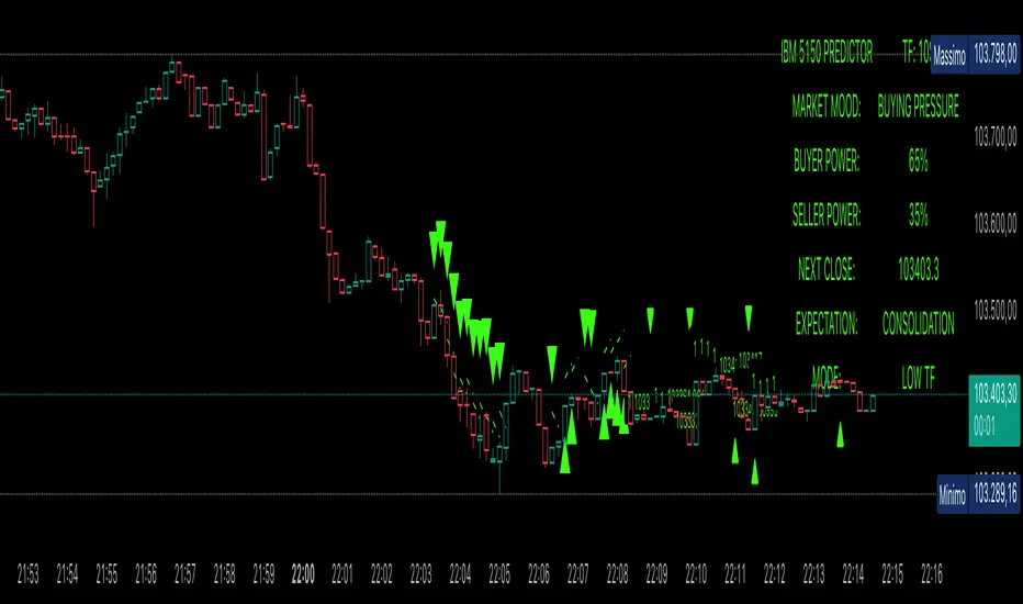
Victoria RSI Hybrid Pro – Momentum + Volume + DivergenceConditions and Actions:
RSI > 50 → Bullish regime → Consider Calls
RSI < 50 → Bearish regime → Consider Puts
RSI crosses up → Momentum shift up → Buy confirmation
RSI crosses down → Momentum shift down → Sell confirmation
RSI > 70 → Overbought → Take profits
RSI < 30 → Oversold → Watch for reversal
Bullish divergence → Hidden upward momentum → Reversal watch
Bearish divergence → Hidden downward momentum → Reversal watch
4. Multi-Indicator Confirmation Rules
Combine signals from EMA, SMA, RSI, and Volume to identify high-confidence trades.
Rules:
Triple Green → EMA1>SMA3, RSI>50, Volume Up → Buy Calls / Shares
Triple Red → EMA1 70 + Weak Volume → Exit Calls early
EMA1 flips direction + Strong Volume → Confirm bias immediately
RSI on 1H agrees with main chart → Trend continuation likely
6. Timeframes
Scalps: 1m–5m
Next-Day Options: 15m–1H
Swings: 4H–1D
7. Key Mindset Rules
Patience beats prediction. Wait for confirmations.
Volume confirms conviction, not direction.
If RSI and Overlay disagree → No trade.
Only act when 2 of 3 systems (EMA, RSI, Volume) align.
chart Pattern & Candle sticks Strategy# **XAUUSD Pattern & Candle Strategy - Complete Description**
## **Overview**
This Pine Script indicator is a comprehensive multi-factor trading system specifically designed for **XAUUSD (Gold) scalping and swing trading**. It combines classical technical analysis methods including candlestick patterns, chart patterns, moving averages, and volume analysis to generate high-probability buy/sell signals with automatic stop-loss and take-profit levels.
***
## **Core Components**
### **1. Moving Average System (Triple MA)**
**Purpose:** Identifies trend direction and momentum
- **Fast MA (20-period)** - Short-term price action
- **Medium MA (50-period)** - Intermediate trend
- **Slow MA (200-period)** - Long-term trend direction
**How it works:**
- **Bullish alignment**: MA20 > MA50 > MA200 (all pointing up)
- **Bearish alignment**: MA20 < MA50 < MA200 (all pointing down)
- **Crossover signals**: When Fast MA crosses Medium MA, it triggers buy/sell signals
- **Choice of SMA or EMA**: Adjustable based on preference
**Visual indicators:**
- Blue line = Fast MA
- Orange line = Medium MA
- Light red line = Slow MA
- Green background tint = Bullish trend
- Red background tint = Bearish trend
---
### **2. Candlestick Pattern Recognition (13 Patterns)**
**Purpose:** Identifies reversal and continuation signals based on price action
#### **Bullish Patterns (Signal potential upward moves):**
1. **Hammer** 🔨
- Long lower wick (2x body size)
- Small body at top
- Indicates rejection of lower prices (buyers stepping in)
- Best at support levels
2. **Inverted Hammer**
- Long upper wick
- Small body at bottom
- Shows buying pressure despite initial selling
3. **Bullish Engulfing** 📈
- Green candle completely engulfs previous red candle
- Strong reversal signal
- Body must be 1.2x larger than previous
4. **Morning Star** ⭐
- 3-candle pattern
- Red candle → Small indecision candle → Large green candle
- Powerful reversal at bottoms
5. **Piercing Line** ⚡
- Green candle closes above 50% of previous red candle
- Indicates strong buying interest
6. **Bullish Marubozu**
- Almost no wicks (95% body)
- Very strong bullish momentum
- Body must be 1.3x average size
#### **Bearish Patterns (Signal potential downward moves):**
7. **Shooting Star** 💫
- Long upper wick
- Small body at bottom
- Indicates rejection of higher prices (sellers in control)
- Best at resistance levels
8. **Hanging Man**
- Similar to hammer but appears at top
- Warning of potential reversal down
9. **Bearish Engulfing** 📉
- Red candle completely engulfs previous green candle
- Strong reversal signal
10. **Evening Star** 🌙
- 3-candle pattern (opposite of Morning Star)
- Green → Small → Large red candle
- Powerful top reversal
11. **Dark Cloud Cover** ☁️
- Red candle closes below 50% of previous green candle
- Indicates strong selling pressure
12. **Bearish Marubozu**
- Almost no wicks, pure red body
- Very strong bearish momentum
#### **Neutral Pattern:**
13. **Doji**
- Open and close nearly equal (tiny body)
- Indicates indecision
- Often precedes major moves
**Detection Logic:**
- Compares body size, wick ratios, and position relative to previous candles
- Uses 14-period average body size as reference
- All patterns validated against volume confirmation
***
### **3. Chart Pattern Recognition**
**Purpose:** Identifies major support/resistance and reversal patterns
#### **Patterns Detected:**
**Double Bottom** 📊 (Bullish)
- Two lows at approximately same level
- Indicates strong support
- Breakout above neckline triggers buy signal
- Most reliable at major support zones
**Double Top** 📊 (Bearish)
- Two highs at approximately same level
- Indicates strong resistance
- Breakdown below neckline triggers sell signal
- Most reliable at major resistance zones
**Support & Resistance Levels**
- Automatically plots recent pivot highs (resistance)
- Automatically plots recent pivot lows (support)
- Uses 3-bar strength for validation
- Levels shown as dashed horizontal lines
**Price Action Patterns**
- **Uptrend detection**: Higher highs + higher lows
- **Downtrend detection**: Lower highs + lower lows
- Confirms overall market structure
***
### **4. Volume Analysis**
**Purpose:** Confirms signal strength and filters false signals
**Metrics tracked:**
- **Volume MA (20-period)**: Baseline average volume
- **High volume threshold**: 1.5x the volume average
- **Volume increase**: Current volume > previous 2 bars
**How it's used:**
- All buy/sell signals **require volume confirmation**
- High volume = institutional participation
- Low volume signals are filtered out
- Prevents whipsaw trades during quiet periods
**Visual indicator:**
- Dashboard shows "High" volume in orange when active
- "Normal" shown in gray during low volume
***
### **5. Signal Generation Logic**
**BUY SIGNALS triggered when ANY of these occur:**
1. **Candlestick + Volume**
- Bullish candle pattern detected
- High volume confirmation
- Price above Fast MA
2. **MA Crossover + Volume**
- Fast MA crosses above Medium MA
- High volume confirmation
3. **Double Bottom Breakout**
- Price breaks above support level
- Volume confirmation present
4. **Trend Continuation**
- Uptrend structure intact (higher highs/lows)
- All MAs in bullish alignment
- Price above Fast MA
- Volume confirmation
**SELL SIGNALS triggered when ANY of these occur:**
1. **Candlestick + Volume**
- Bearish candle pattern detected
- High volume confirmation
- Price below Fast MA
2. **MA Crossunder + Volume**
- Fast MA crosses below Medium MA
- High volume confirmation
3. **Double Top Breakdown**
- Price breaks below resistance level
- Volume confirmation present
4. **Trend Continuation**
- Downtrend structure intact (lower highs/lows)
- All MAs in bearish alignment
- Price below Fast MA
- Volume confirmation
***
### **6. Risk Management System**
**Automatic Stop Loss Calculation:**
- Based on ATR (Average True Range) - 14 periods
- **Formula**: Entry price ± (ATR × SL Multiplier)
- **Default multiplier**: 1.5 (adjustable)
- Adapts to market volatility automatically
**Automatic Take Profit Calculation:**
- **Formula**: Entry price ± (ATR × TP Multiplier)
- **Default multiplier**: 2.5 (adjustable)
- **Default Risk:Reward ratio**: 1:1.67
- Higher TP multiplier = more aggressive targets
**Position Management:**
- Tracks ONE position at a time (no pyramiding)
- Automatically closes position when:
- Stop loss is hit
- Take profit is reached
- Opposite MA crossover occurs
- Prevents revenge trading and over-leveraging
**Visual Representation:**
- **Red horizontal line** = Stop Loss level
- **Green horizontal line** = Take Profit level
- Lines remain on chart while position is active
- Automatically disappear when position closes
***
### **7. Visual Elements**
**On-Chart Displays:**
1. **Moving Average Lines**
- Fast MA (Blue, thick)
- Medium MA (Orange, thick)
- Slow MA (Red, thin)
2. **Support/Resistance**
- Green crosses = Support levels
- Red crosses = Resistance levels
3. **Buy/Sell Arrows**
- Large GREEN "BUY" label below bars
- Large RED "SELL" label above bars
4. **Pattern Labels** (Small markers)
- "Hammer", "Bull Engulf", "Morning Star" (green, below bars)
- "Shooting Star", "Bear Engulf", "Evening Star" (red, above bars)
- "Double Bottom" / "Double Top" (blue/orange)
5. **Signal Detail Labels** (Medium size)
- Shows signal reason (e.g., "Bullish Candle", "MA Cross Up")
- Displays Entry, SL, and TP prices
- Color-coded (green for long, red for short)
6. **Background Coloring**
- Light green tint = Bullish MA alignment
- Light red tint = Bearish MA alignment
***
### **8. Information Dashboard**
**Top-right corner table showing:**
| Metric | Description |
|--------|-------------|
| **Position** | Current trade status (LONG/SHORT/None) |
| **MA Trend** | Overall trend direction (Bullish/Bearish/Neutral) |
| **Volume** | Current volume status (High/Normal) |
| **Pattern** | Last detected candlestick pattern |
| **ATR** | Current volatility measurement |
**Purpose:**
- Quick at-a-glance market assessment
- Real-time position tracking
- No need to check multiple indicators
***
### **9. Alert System**
**Complete alert coverage for:**
✅ **Entry Alerts**
- "Buy Signal" - Triggers when buy conditions met
- "Sell Signal" - Triggers when sell conditions met
✅ **Exit Alerts**
- "Long TP Hit" - Take profit reached on long position
- "Long SL Hit" - Stop loss triggered on long position
- "Short TP Hit" - Take profit reached on short position
- "Short SL Hit" - Stop loss triggered on short position
**How to use:**
1. Click "Create Alert" button
2. Select desired alert from dropdown
3. Set notification method (popup, email, SMS, webhook)
4. Never miss a trade opportunity
***
## **Recommended Settings**
### **For Scalping (Quick trades):**
- **Timeframe**: 5-minute
- **Fast MA**: 9
- **Medium MA**: 21
- **Slow MA**: 50
- **SL Multiplier**: 1.0
- **TP Multiplier**: 2.0
- **Volume Threshold**: 1.5x
### **For Swing Trading (Longer holds):**
- **Timeframe**: 1-hour or 4-hour
- **Fast MA**: 20
- **Medium MA**: 50
- **Slow MA**: 200
- **SL Multiplier**: 2.0
- **TP Multiplier**: 3.0
- **Volume Threshold**: 1.3x
### **Best Trading Hours for XAUUSD:**
- **Asian Session**: 00:00 - 08:00 GMT (lower volatility)
- **London Session**: 08:00 - 16:00 GMT (high volatility) ⭐
- **New York Session**: 13:00 - 21:00 GMT (highest volume) ⭐
- **London-NY Overlap**: 13:00 - 16:00 GMT (BEST for scalping) 🔥
***
## **How to Use This Strategy**
### **Step 1: Setup**
1. Open TradingView
2. Load XAUUSD chart
3. Select timeframe (5m, 15m, 1H, or 4H)
4. Add indicator from Pine Editor
5. Adjust settings based on your trading style
### **Step 2: Wait for Signals**
- Watch for GREEN "BUY" or RED "SELL" labels
- Check the signal reason in the detail label
- Verify dashboard shows favorable conditions
- Confirm volume is "High" (not required but preferred)
### **Step 3: Enter Trade**
- Enter at market or limit order near signal price
- Note the displayed Entry, SL, and TP prices
- Set your broker's SL/TP to match indicator levels
### **Step 4: Manage Position**
- Watch for SL/TP lines on chart
- Monitor dashboard for trend changes
- Exit manually if opposite MA crossover occurs
- Let SL/TP do their job (don't move them!)
### **Step 5: Review & Learn**
- Track win rate over 20+ trades
- Adjust multipliers if needed
- Note which patterns work best for you
- Refine entry timing
***
## **Key Advantages**
✅ **Multi-confirmation approach** - Reduces false signals significantly
✅ **Automatic risk management** - No manual calculation needed
✅ **Adapts to volatility** - ATR-based SL/TP adjusts to market conditions
✅ **Volume filtered** - Ensures institutional participation
✅ **Visual clarity** - Easy to understand at a glance
✅ **Complete alert system** - Never miss opportunities
✅ **Pattern education** - Learn patterns as they appear
✅ **Works on all timeframes** - Scalping to swing trading
***
## **Limitations & Considerations**
⚠️ **Not a holy grail** - No strategy wins 100% of trades
⚠️ **Requires practice** - Demo trade first to understand signals
⚠️ **Market conditions matter** - Works best in trending or volatile markets
⚠️ **News events** - Avoid trading during major economic releases
⚠️ **Slippage on 5m** - Fast markets may have execution delays
⚠️ **Pattern subjectivity** - Some patterns may trigger differently than expected
***
## **Risk Management Rules**
1. **Never risk more than 1-2% per trade**
2. **Maximum 3 positions per day** (avoid overtrading)
3. **Don't trade during major news** (NFP, FOMC, etc.)
4. **Use proper position sizing** (0.01 lot per $100 for micro accounts)
5. **Keep trade journal** (track patterns, win rate, mistakes)
6. **Stop trading after 3 consecutive losses** (psychological reset)
7. **Don't move stop loss further away** (accept losses)
8. **Take partial profits** at 1:1 R:R if desired
***
## **Expected Performance**
**Realistic expectations:**
- **Win rate**: 50-65% (depending on market conditions and timeframe)
- **Risk:Reward**: 1:1.67 default (adjustable to 1:2 or 1:3)
- **Signals per day**: 3-8 on 5m, 1-3 on 1H
- **Best months**: High volatility periods (news events, economic uncertainty)
- **Drawdowns**: Expect 3-5 losing trades in a row occasionally
***
## **Customization Options**
All inputs are adjustable in settings panel:
**Moving Averages:**
- Type (SMA or EMA)
- All three period lengths
**Volume:**
- Volume MA length
- High volume multiplier threshold
**Chart Patterns:**
- Pattern strength (bars for pivot detection)
- Show/hide pattern labels
**Risk Management:**
- ATR period
- Stop loss multiplier
- Take profit multiplier
**Display:**
- Toggle pattern labels
- Customize colors (in code)
***
## **Conclusion**
This is a **professional-grade, multi-factor trading system** that combines the best of classical technical analysis with modern risk management. It's designed to give clear, actionable signals while automatically handling the complex calculations of stop loss and take profit levels.
**Best suited for traders who:**
- Understand basic technical analysis
- Can follow rules consistently
- Prefer systematic approach over gut feeling
- Want visual confirmation before entering trades
- Value proper risk management
**Start with demo trading** for at least 20-30 trades to understand how the signals work in different market conditions. Once comfortable and profitable on demo, transition to live trading with minimal risk per trade.
Happy trading! 📈🎯

MCL RSI Conflux v2.5 — Multi-Timeframe Momentum & Z-Score Full Description
Overview
The MCL RSI Conflux v2.5 is a multi-timeframe momentum model that integrates daily, weekly, and monthly RSI values into a unified composite. It extends the classical RSI framework with adaptive overbought/oversold thresholds and statistical normalization (Z-score confluence).
This combination allows traders to visualize cross-timeframe alignment, identify synchronized momentum shifts, and detect exhaustion zones with higher statistical confidence.
Methodology
The script extracts RSI data from three major time horizons:
Daily RSI (short-term momentum)
Weekly RSI (intermediate trend)
Monthly RSI (macro bias)
Each RSI is optionally smoothed, weighted, and aggregated into a Composite RSI.
A Z-score transformation then measures how far each RSI deviates from its historical mean, revealing when momentum strength is statistically extreme or aligned across timeframes.
Key Features
Multi-Timeframe RSI Engine – Computes RSI across D/W/M intervals with individual weighting controls.
Adaptive Overbought/Oversold Bands – Automatically adjusts OB/OS thresholds based on rolling volatility (standard deviation of daily RSI).
Composite RSI Score – Weighted consensus RSI that represents total market momentum.
Z-Score Confluence Analysis – Identifies when all three timeframes are statistically synchronized.
Z-Composite Histogram – Displays aggregated Z-score strength around the midline (50).
Divergence Detection – Flags confirmed pivot-based bull and bear divergences on the daily RSI.
Dynamic Gradient Background – Shifts from red to green based on composite momentum regime.
Customizable Control Panel – Displays RSI values, Z-scores, state, and adaptive bands for each timeframe.
Integrated Alerts – For crossovers, risk-on/off thresholds, alignment, and Z-confluence events.
Interpretation
All RSI values above 50: multi-timeframe bullish alignment.
All RSI values below 50: multi-timeframe bearish alignment.
Composite RSI > 60: risk-on environment; momentum expansion.
Composite RSI < 45: risk-off environment; momentum contraction.
Adaptive OB/OS hits: potential exhaustion or mean reversion setup.
Green Z-ribbon: all Z-scores positive and aligned (statistical confirmation).
Red Z-ribbon: all Z-scores negative and aligned (broad market weakness).
Divergences: short-term warning signals against the prevailing momentum bias.
Practical Application
Use the Composite RSI as a global momentum gauge for position bias.
Trade only in the direction of higher-timeframe alignment (avoid countertrend RSI).
Combine Z-ribbon confirmation with Composite RSI crosses to filter noise.
Use divergence labels and adaptive thresholds for risk reduction or exit timing.
Ideal for swing traders and macro momentum models seeking trend synchronization filters.
Recommended Settings
Market Mode k-Band Lookback Use Case
Stocks / ETFs Adaptive 0.85 200 Medium-term rotation filter
Crypto Adaptive 1.00 150 Volatility-responsive swing filter
Commodities Fixed 70/30 100 Mean reversion model
Alerts Included
Daily RSI crossed above/below Weekly RSI
Composite RSI > Risk-On threshold
Composite RSI < Risk-Off threshold
All RSI aligned above/below 50
Z-Score Conformity (All positive or all negative)
Overbought/Oversold triggers
Author’s Note
This indicator was designed for research and systematic confluence analysis within Mongoose Capital Labs.
It is not financial advice and should be used in combination with independent risk assessment, volume confirmation, and higher-timeframe context.

3D Institutional Battlefield [SurgeGuru]Professional Presentation: 3D Institutional Flow Terrain Indicator
Overview
The 3D Institutional Flow Terrain is an advanced trading visualization tool that transforms complex market structure into an intuitive 3D landscape. This indicator synthesizes multiple institutional data points—volume profiles, order blocks, liquidity zones, and voids—into a single comprehensive view, helping you identify high-probability trading opportunities.
Key Features
🎥 Camera & Projection Controls
Yaw & Pitch: Adjust viewing angles (0-90°) for optimal perspective
Scale Controls: Fine-tune X (width), Y (depth), and Z (height) dimensions
Pro Tip: Increase Z-scale to amplify terrain features for better visibility
🌐 Grid & Surface Configuration
Resolution: Adjust X (16-64) and Y (12-48) grid density
Visual Elements: Toggle surface fill, wireframe, and node markers
Optimization: Higher resolution provides more detail but requires more processing power
📊 Data Integration
Lookback Period: 50-500 bars of historical analysis
Multi-Source Data: Combine volume profile, order blocks, liquidity zones, and voids
Weighted Analysis: Each data source contributes proportionally to the terrain height
How to Use the Frontend
💛 Price Line Tracking (Your Primary Focus)
The yellow price line is your most important guide:
Monitor Price Movement: Track how the yellow line interacts with the 3D terrain
Identify Key Levels: Watch for these critical interactions:
Order Blocks (Green/Red Zones):
When yellow price line enters green zones = Bullish order block
When yellow price line enters red zones = Bearish order block
These represent institutional accumulation/distribution areas
Liquidity Voids (Yellow Zones):
When yellow price line enters yellow void areas = Potential acceleration zones
Voids indicate price gaps where minimal trading occurred
Price often moves rapidly through voids toward next liquidity pool
Terrain Reading:
High Terrain Peaks: High volume/interest areas (support/resistance)
Low Terrain Valleys: Low volume areas (potential breakout zones)
Color Coding:
Green terrain = Bullish volume dominance
Red terrain = Bearish volume dominance
Purple = Neutral/transition areas
📈 Volume Profile Integration
POC (Point of Control): Automatically marks highest volume level
Volume Bins: Adjust granularity (10-50 bins)
Height Weight: Control how much volume affects terrain elevation
🏛️ Order Block Detection
Detection Length: 5-50 bar lookback for block identification
Strength Weighting: Recent blocks have greater impact on terrain
Candle Body Option: Use full candles or body-only for block definition
💧 Liquidity Zone Tracking
Multiple Levels: Track 3-10 key liquidity zones
Buy/Sell Side: Different colors for bid/ask liquidity
Strength Decay: Older zones have diminishing terrain impact
🌊 Liquidity Void Identification
Threshold Multiplier: Adjust sensitivity (0.5-2.0)
Height Amplification: Voids create significant terrain depressions
Acceleration Zones: Price typically moves quickly through void areas
Practical Trading Application
Bullish Scenario:
Yellow price line approaches green order block terrain
Price finds support in elevated bullish volume areas
Terrain shows consistent elevation through key levels
Bearish Scenario:
Yellow price line struggles at red order block resistance
Price falls through liquidity voids toward lower terrain
Bearish volume peaks dominate the landscape
Breakout Setup:
Yellow price line consolidates in flat terrain
Minimal resistance (low terrain) in projected direction
Clear path toward distant liquidity zones
Pro Tips
Start Simple: Begin with default settings, then gradually customize
Focus on Yellow Line: Your primary indicator of current price position
Combine Timeframes: Use the same terrain across multiple timeframes for confluence
Volume Confirmation: Ensure terrain peaks align with actual volume spikes
Void Anticipation: When price enters voids, prepare for potential rapid movement
Order Blocks & Voids Architecture
Order Blocks Calculation
Trigger: Price breaks fractal swing points
Bullish OB: When close > swing high → find lowest low in lookback period
Bearish OB: When close < swing low → find highest high in lookback period
Strength: Based on price distance from block extremes
Storage: Global array maintains last 50 blocks with FIFO management
Liquidity Voids Detection
Trigger: Price gaps exceeding ATR threshold
Bull Void: Low - high > (ATR200 × multiplier)
Bear Void: Low - high > (ATR200 × multiplier)
Validation: Close confirms gap direction
Storage: Global array maintains last 30 voids
Key Design Features
Real-time Updates: Calculated every bar, not just on last bar
Global Persistence: Arrays maintain state across executions
FIFO Management: Automatic cleanup of oldest entries
Configurable Sensitivity: Adjustable lookback periods and thresholds
Scientific Testing Framework
Hypothesis Testing
Primary Hypothesis: 3D terrain visualization improves detection of institutional order flow vs traditional 2D charts
Testable Metrics:
Prediction Accuracy: Does terrain structure predict future support/resistance?
Reaction Time: Faster identification of key levels vs conventional methods
False Positive Reduction: Lower rate of failed breakouts/breakdowns
Control Variables
Market Regime: Trending vs ranging conditions
Asset Classes: Forex, equities, cryptocurrencies
Timeframes: M5 to H4 for intraday, D1 for swing
Volume Conditions: High vs low volume environments
Data Collection Protocol
Terrain Features to Quantify:
Slope gradient changes at price inflection points
Volume peak clustering density
Order block terrain elevation vs subsequent price action
Void depth correlation with momentum acceleration
Control Group: Traditional support/resistance + volume profile
Experimental Group: 3D Institutional Flow Terrain
Statistical Measures
Signal-to-Noise Ratio: Terrain features vs random price movements
Lead Time: Terrain formation ahead of price confirmation
Effect Size: Performance difference between groups (Cohen's d)
Statistical Power: Sample size requirements for significance
Validation Methodology
Blind Testing:
Remove price labels from terrain screenshots
Have traders identify key levels from terrain alone
Measure accuracy vs actual price action
Backtesting Framework:
Automated terrain feature extraction
Correlation with future price reversals/breakouts
Monte Carlo simulation for significance testing
Expected Outcomes
If hypothesis valid:
Significant improvement in level prediction accuracy (p < 0.05)
Reduced latency in institutional level identification
Higher risk-reward ratios on terrain-confirmed trades
Research Questions:
Does terrain elevation reliably indicate institutional interest zones?
Are liquidity voids statistically significant momentum predictors?
Does multi-timeframe terrain analysis improve signal quality?
How does terrain persistence correlate with level strength?
LuxAlgo BigBeluga hapharmonic

🔥 QUANT MOMENTUM SKORQUANT MOMENTUM SCORE – Description (EN)
Summary: This indicator fuses Price ROC, RSI, MACD, Trend Strength (ADX+EMA) and Volume into a single 0-100 “Momentum Score.” Guide bands (50/60/70/80) and ready-to-use alert conditions are included.
How it works
Price Momentum (ROC): Rate of change normalized to 0-100.
RSI Momentum: RSI treated as a momentum proxy and mapped to 0-100.
MACD Momentum: MACD histogram normalized to capture acceleration.
Trend Strength: ADX is direction-aware (DI+ vs DI–) and blended with EMA state (above/below) to form a combined trend score.
Volume Momentum: Volume relative to its moving average (ratio-based).
Weighting: All five components are weighted, auto-normalized, and summed into the final 0-100 score.
Visuals & Alerts: Score line with 50/60/70/80 guides; threshold-cross alerts for High/Strong/Ultra-Strong regimes.
Inputs, weights and thresholds are configurable; total weights are normalized automatically.
How to use
Timeframes: Works on any timeframe—lower TFs react faster; higher TFs reduce noise.
Reading the score:
<50: Weak momentum
50-60: Transition
60-70: Moderate-Strong (potential acceleration)
≥70: Strong, ≥80: Ultra Strong
Practical tip: Use it as a filter, not a stand-alone signal. Combine score breakouts with market structure/trend context (e.g., pullback-then-re-acceleration) to improve selectivity.
Disclaimer: This is not financial advice; past performance does not guarantee future results.

TrendFlowTrendFlow is a visual trend analysis tool that helps identify changes in market direction and momentum.
It uses three exponential moving averages (EMA 21, EMA 50, and EMA 200) to define short-, medium-, and long-term trend structure.
A dynamic color fill highlights the relationship between the 21 and 50 EMAs:
When EMA 21 is above EMA 50, a green fill indicates upward momentum.
When EMA 21 is below EMA 50, a red fill shows downward momentum.
The EMA 200 line adapts its color based on its position relative to the shorter EMAs:
Red when above both EMAs (strong upward structure)
Green when below both EMAs (strong downward structure)
Gray when between them (neutral or consolidation phase)
This setup provides a clear visual framework for observing trend flow and directional bias over multiple timeframes.
Developed by The Volume Hub Fintech and Strategy Development
