[blackcat] L2 Ehlers Adaptive Commodity Channel IndexLevel: 2
Background
John F. Ehlers introucedAdaptive Commodity Channel Index in his "Rocket Science for Traders" chapter 21 on 2001.
Function
The Commodity Channel Index (CCI) computes the average of the median price of each bar over the observation period. It also computes the Mean Deviation (MD) from this average. The CCI is formed as the current deviation from the average price normalized to the MD. With a Gaussian probability distribution, 68 percent of all possible outcomes are contained within the first standard deviation from the mean. The CCI is scaled so that values above +l00 are above the upper first
standard deviation from the mean and values below -100 are below the lower first standard deviation from the mean. Multiplying the MD in the code by 0.015 implements this normalization. Many traders use this indicator as an overbought/oversold indicator with 100 or greater indicating that the market is overbought, and -100 or less that the market is oversold. Since the trading channel is being formed by the indicator, the obvious observation period is the same as the cycle length. Since the complete cycle period may not be the universal answer, Dr. Ehlers includes a CycPart input as a modifier. This input allows you to optimize the observation period for each particular situation.
Key Signal
CCI ---> Adaptive Commodity Channel Index fast line
CCI ---> Adaptive Commodity Channel Index slow line
Pros and Cons
100% John F. Ehlers definition translation of original work, even variable names are the same. This help readers who would like to use pine to read his book. If you had read his works, then you will be quite familiar with my code style.
Remarks
The 20th script for Blackcat1402 John F. Ehlers Week publication.
Readme
In real life, I am a prolific inventor. I have successfully applied for more than 60 international and regional patents in the past 12 years. But in the past two years or so, I have tried to transfer my creativity to the development of trading strategies. Tradingview is the ideal platform for me. I am selecting and contributing some of the hundreds of scripts to publish in Tradingview community. Welcome everyone to interact with me to discuss these interesting pine scripts.
The scripts posted are categorized into 5 levels according to my efforts or manhours put into these works.
Level 1 : interesting script snippets or distinctive improvement from classic indicators or strategy. Level 1 scripts can usually appear in more complex indicators as a function module or element.
Level 2 : composite indicator/strategy. By selecting or combining several independent or dependent functions or sub indicators in proper way, the composite script exhibits a resonance phenomenon which can filter out noise or fake trading signal to enhance trading confidence level.
Level 3 : comprehensive indicator/strategy. They are simple trading systems based on my strategies. They are commonly containing several or all of entry signal, close signal, stop loss, take profit, re-entry, risk management, and position sizing techniques. Even some interesting fundamental and mass psychological aspects are incorporated.
Level 4 : script snippets or functions that do not disclose source code. Interesting element that can reveal market laws and work as raw material for indicators and strategies. If you find Level 1~2 scripts are helpful, Level 4 is a private version that took me far more efforts to develop.
Level 5 : indicator/strategy that do not disclose source code. private version of Level 3 script with my accumulated script processing skills or a large number of custom functions. I had a private function library built in past two years. Level 5 scripts use many of them to achieve private trading strategy.
스크립트에서 "中国铝业2001年股价"에 대해 찾기
[blackcat] L2 Ehlers Adaptive StochasticLevel: 2
Background
John F. Ehlers introuced Adaptive Stochastic in his "Rocket Science for Traders" chapter 21 on 2001.
Function
The Stochastic measures the current closing price relative to the lowest low over the observation period. It then normalizes this to the range between the highest high and the lowest low over the observation period. If the current closing price is equal to the highest high over the observation period, then the Stochastic has a value of 1. If the current closing price is equal to the lowest low over the observation period, then the Stochastic has a value of zero. These are the limits over which the Stochastic can range. To optimize the Stochastic for the measured cycle, the correct fraction of the cycle to use is one-half, as the Stochastic can
range from its minimum to its maximum on each half cycle of the period. As before, the code for the optimized Stochastic measures the cycle period using the Homodyne Discriminator algorithm and then uses that period as the basis for finding HH and LL and computing the Stochastic. Since half the cycle period may not be the universal answer, we include a CycPart input as a modifier. This input allows you to optimize the observation period for each particular situation. The optimized Stochastic tends to be in phase with the original price data. This suggests a way to turn a good indicator into a great one. If we subtract 50 from the optimized Stochastic, we would get a zero mean and thus tend to have Poisson-like statistics on the Stochastic’s zero crossings. If that were the case, we could smooth the optimized Stochastic and make an Optimum Predictive filter from it. That way we could anticipate signals rather than wait for signals to cross the 20 percent and 80 percent marks for confirmation as is done with the standard indicator. I will leave it to you to decide which method best suits your needs and purposes.
Key Signal
Stochastic ---> Stochastic fast line
Stochastic ---> Stochastic slow line
Pros and Cons
100% John F. Ehlers definition translation of original work, even variable names are the same. This help readers who would like to use pine to read his book. If you had read his works, then you will be quite familiar with my code style.
Remarks
The 19th script for Blackcat1402 John F. Ehlers Week publication.
Readme
In real life, I am a prolific inventor. I have successfully applied for more than 60 international and regional patents in the past 12 years. But in the past two years or so, I have tried to transfer my creativity to the development of trading strategies. Tradingview is the ideal platform for me. I am selecting and contributing some of the hundreds of scripts to publish in Tradingview community. Welcome everyone to interact with me to discuss these interesting pine scripts.
The scripts posted are categorized into 5 levels according to my efforts or manhours put into these works.
Level 1 : interesting script snippets or distinctive improvement from classic indicators or strategy. Level 1 scripts can usually appear in more complex indicators as a function module or element.
Level 2 : composite indicator/strategy. By selecting or combining several independent or dependent functions or sub indicators in proper way, the composite script exhibits a resonance phenomenon which can filter out noise or fake trading signal to enhance trading confidence level.
Level 3 : comprehensive indicator/strategy. They are simple trading systems based on my strategies. They are commonly containing several or all of entry signal, close signal, stop loss, take profit, re-entry, risk management, and position sizing techniques. Even some interesting fundamental and mass psychological aspects are incorporated.
Level 4 : script snippets or functions that do not disclose source code. Interesting element that can reveal market laws and work as raw material for indicators and strategies. If you find Level 1~2 scripts are helpful, Level 4 is a private version that took me far more efforts to develop.
Level 5 : indicator/strategy that do not disclose source code. private version of Level 3 script with my accumulated script processing skills or a large number of custom functions. I had a private function library built in past two years. Level 5 scripts use many of them to achieve private trading strategy.

[blackcat] L2 Ehlers Adaptive Relative Strength IndexLevel: 2
Background
John F. Ehlers introuced Adaptive Relative Strength Index in his "Rocket Science for Traders" chapter 21 on 2001.
Function
The concept of taking a difference of lagging line from the original function to produce a leading function suggests extending the concept to moving averages. There is no direct theory for this, but it seems to work pretty well. If taking a 7-bar WMA of prices, that average lags the prices by 2 bars. If taking a 7-bar WMA of the first average, this second average is delayed another 2 bars. If taking the difference between the two averages and add that difference to the first average, the result should be a smoothed line of the original price function with no lag. Sure, Dr. Ehlers tried to use more lag for the second moving average, which
should produce a better predictive curve. However, remember the lesson of Chapter 3 of the book. An analysis curve cannot precede an event. You cannot predict an event before it occurs. If then taking a 4-bar WMA of the smoothed line to create a 1-bar lag, this lagging line becomes a signal when the lines cross. This is as close to an ideal indicator as we can get.
Key Signal
Predict ---> moving average fast line
Trigger ---> moving average slow line
Pros and Cons
100% John F. Ehlers definition translation of original work, even variable names are the same. This help readers who would like to use pine to read his book. If you had read his works, then you will be quite familiar with my code style.
Remarks
The 17th script for Blackcat1402 John F. Ehlers Week publication.
Readme
In real life, I am a prolific inventor. I have successfully applied for more than 60 international and regional patents in the past 12 years. But in the past two years or so, I have tried to transfer my creativity to the development of trading strategies. Tradingview is the ideal platform for me. I am selecting and contributing some of the hundreds of scripts to publish in Tradingview community. Welcome everyone to interact with me to discuss these interesting pine scripts.
The scripts posted are categorized into 5 levels according to my efforts or manhours put into these works.
Level 1 : interesting script snippets or distinctive improvement from classic indicators or strategy. Level 1 scripts can usually appear in more complex indicators as a function module or element.
Level 2 : composite indicator/strategy. By selecting or combining several independent or dependent functions or sub indicators in proper way, the composite script exhibits a resonance phenomenon which can filter out noise or fake trading signal to enhance trading confidence level.
Level 3 : comprehensive indicator/strategy. They are simple trading systems based on my strategies. They are commonly containing several or all of entry signal, close signal, stop loss, take profit, re-entry, risk management, and position sizing techniques. Even some interesting fundamental and mass psychological aspects are incorporated.
Level 4 : script snippets or functions that do not disclose source code. Interesting element that can reveal market laws and work as raw material for indicators and strategies. If you find Level 1~2 scripts are helpful, Level 4 is a private version that took me far more efforts to develop.
Level 5 : indicator/strategy that do not disclose source code. private version of Level 3 script with my accumulated script processing skills or a large number of custom functions. I had a private function library built in past two years. Level 5 scripts use many of them to achieve private trading strategy.

[blackcat] L2 Ehlers Predictive AverageLevel: 2
Background
John F. Ehlers introuced Predictive Average in his "Rocket Science for Traders" chapter 20 on 2001.
Function
The concept of taking a difference of lagging line from the original function to produce a leading function suggests extending the concept to moving averages. There is no direct theory for this, but it seems to work pretty well. If taking a 7-bar WMA of prices, that average lags the prices by 2 bars. If taking a 7-bar WMA of the first average, this second average is delayed another 2 bars. If taking the difference between the two averages and add that difference to the first average, the result should be a smoothed line of the original price function with no lag. Sure, Dr. Ehlers tried to use more lag for the second moving average, which
should produce a better predictive curve. However, remember the lesson of Chapter 3 of the book. An analysis curve cannot precede an event. You cannot predict an event before it occurs. If then taking a 4-bar WMA of the smoothed line to create a 1-bar lag, this lagging line becomes a signal when the lines cross. This is as close to an ideal indicator as we can get.
Key Signal
Predict ---> moving average fast line
Trigger ---> moving average slow line
Pros and Cons
100% John F. Ehlers definition translation of original work, even variable names are the same. This help readers who would like to use pine to read his book. If you had read his works, then you will be quite familiar with my code style.
Remarks
The 17th script for Blackcat1402 John F. Ehlers Week publication.
Readme
In real life, I am a prolific inventor. I have successfully applied for more than 60 international and regional patents in the past 12 years. But in the past two years or so, I have tried to transfer my creativity to the development of trading strategies. Tradingview is the ideal platform for me. I am selecting and contributing some of the hundreds of scripts to publish in Tradingview community. Welcome everyone to interact with me to discuss these interesting pine scripts.
The scripts posted are categorized into 5 levels according to my efforts or manhours put into these works.
Level 1 : interesting script snippets or distinctive improvement from classic indicators or strategy. Level 1 scripts can usually appear in more complex indicators as a function module or element.
Level 2 : composite indicator/strategy. By selecting or combining several independent or dependent functions or sub indicators in proper way, the composite script exhibits a resonance phenomenon which can filter out noise or fake trading signal to enhance trading confidence level.
Level 3 : comprehensive indicator/strategy. They are simple trading systems based on my strategies. They are commonly containing several or all of entry signal, close signal, stop loss, take profit, re-entry, risk management, and position sizing techniques. Even some interesting fundamental and mass psychological aspects are incorporated.
Level 4 : script snippets or functions that do not disclose source code. Interesting element that can reveal market laws and work as raw material for indicators and strategies. If you find Level 1~2 scripts are helpful, Level 4 is a private version that took me far more efforts to develop.
Level 5 : indicator/strategy that do not disclose source code. private version of Level 3 script with my accumulated script processing skills or a large number of custom functions. I had a private function library built in past two years. Level 5 scripts use many of them to achieve private trading strategy.

[blackcat] L2 Ehlers Optimum PredictorLevel: 2
Background
John F. Ehlers introuced Optimum Predictor in his "Rocket Science for Traders" chapter 20 on 2001.
Function
As we have seen before, the majority of the code involves the computation of the period using the Homodyne Discriminator algorithm. Once the period has
been computed, the Optimum Predictor is found in just a few lines of code. First, the minimum-length Hilbert Transformer is used to compute the Detrender2 value from the prices that have been smoothed by the 4-bar Weighted Moving Average (WMA). Detrender2 is smoothed in the 4-bar WMA to produce Smooth2. The alpha of the EMA is computed from the computed period, and the EMA of Smooth2 is taken using that alpha and is called the DetrendEMA. The difference between Smooth2 and the
DetrendEMA is multiplied by 1.4 to produce the Predict phasor. Finally, the Smooth2 and Predict phasors are plotted as indicators.
The Optimum Predictor is plotted as the subgraph below the price chart. Buy and sell signals occur when the Predict and Smooth2 lines cross. Based on Dr. Ehlers comments, most of these signals are indeed prescient. The Optimum Predictor could probably work best in trading systems when used in conjunction with other
rules to eliminate the false signals.
Key Signal
Smooth --> 4 bar WMA w/ 1 bar lag
Detrender --> The amplitude response of a minimum-length HT can be improved by adjusting the filter coefficients by
trial and error. HT does not allow DC component at zero frequency for transformation. So, Detrender is used to remove DC component/ trend component.
Q1 --> Quadrature phase signal
I1 --> In-phase signal
Period --> Dominant Cycle in bars
SmoothPeriod --> Period with complex averaging
Predict --> fast line of optimum predictor
Smooth2 --> slow line of optimum predictor
Pros and Cons
100% John F. Ehlers definition translation of original work, even variable names are the same. This help readers who would like to use pine to read his book. If you had read his works, then you will be quite familiar with my code style.
Remarks
The 16th script for Blackcat1402 John F. Ehlers Week publication.
Readme
In real life, I am a prolific inventor. I have successfully applied for more than 60 international and regional patents in the past 12 years. But in the past two years or so, I have tried to transfer my creativity to the development of trading strategies. Tradingview is the ideal platform for me. I am selecting and contributing some of the hundreds of scripts to publish in Tradingview community. Welcome everyone to interact with me to discuss these interesting pine scripts.
The scripts posted are categorized into 5 levels according to my efforts or manhours put into these works.
Level 1 : interesting script snippets or distinctive improvement from classic indicators or strategy. Level 1 scripts can usually appear in more complex indicators as a function module or element.
Level 2 : composite indicator/strategy. By selecting or combining several independent or dependent functions or sub indicators in proper way, the composite script exhibits a resonance phenomenon which can filter out noise or fake trading signal to enhance trading confidence level.
Level 3 : comprehensive indicator/strategy. They are simple trading systems based on my strategies. They are commonly containing several or all of entry signal, close signal, stop loss, take profit, re-entry, risk management, and position sizing techniques. Even some interesting fundamental and mass psychological aspects are incorporated.
Level 4 : script snippets or functions that do not disclose source code. Interesting element that can reveal market laws and work as raw material for indicators and strategies. If you find Level 1~2 scripts are helpful, Level 4 is a private version that took me far more efforts to develop.
Level 5 : indicator/strategy that do not disclose source code. private version of Level 3 script with my accumulated script processing skills or a large number of custom functions. I had a private function library built in past two years. Level 5 scripts use many of them to achieve private trading strategy.

[blackcat] L2 The Distance Coefficient Ehlers FilterLevel: 2
Background
John F. Ehlers introuced the Distance Coefficient Ehlers Filter in his "Rocket Science for Traders" chapter 18 on 2001.
Function
Dr. Ehlers considered the gray shading levels as distances, he had away of computing filter coefficients in terms of sharpness of the edge. White is the maximum distance in one direction from the median gray, and black is the maximum distance in the other direction. In this sense, distance is a measure of departure from the edge, taking into account the edge sharpness. Transitioning to price charts, the difference in prices can be imagined as a distance. Recalling the Pythagorean Theorem (which the length of the hypotenuse of a triangle is equal to the sum of the squares of the lengths of the other two sides), Dr Ehlers applied it to the needs and say that a generalized length at any data sample is the square root of the sum of the squares of the price difference between that price and each of the prices back for the length of the filter window. The distances squared at each data point are the coefficients of the Ehlers filter.
Key Signal
Coef --> Ehlers filter coefficients array
Distance2 --> Distance array
Filt --> Ehlers filter output
Pros and Cons
100% John F. Ehlers definition translation of original work, even variable names are the same. This help readers who would like to use pine to read his book. If you had read his works, then you will be quite familiar with my code style.
Remarks
The 15th script for Blackcat1402 John F. Ehlers Week publication.
Readme
In real life, I am a prolific inventor. I have successfully applied for more than 60 international and regional patents in the past 12 years. But in the past two years or so, I have tried to transfer my creativity to the development of trading strategies. Tradingview is the ideal platform for me. I am selecting and contributing some of the hundreds of scripts to publish in Tradingview community. Welcome everyone to interact with me to discuss these interesting pine scripts.
The scripts posted are categorized into 5 levels according to my efforts or manhours put into these works.
Level 1 : interesting script snippets or distinctive improvement from classic indicators or strategy. Level 1 scripts can usually appear in more complex indicators as a function module or element.
Level 2 : composite indicator/strategy. By selecting or combining several independent or dependent functions or sub indicators in proper way, the composite script exhibits a resonance phenomenon which can filter out noise or fake trading signal to enhance trading confidence level.
Level 3 : comprehensive indicator/strategy. They are simple trading systems based on my strategies. They are commonly containing several or all of entry signal, close signal, stop loss, take profit, re-entry, risk management, and position sizing techniques. Even some interesting fundamental and mass psychological aspects are incorporated.
Level 4 : script snippets or functions that do not disclose source code. Interesting element that can reveal market laws and work as raw material for indicators and strategies. If you find Level 1~2 scripts are helpful, Level 4 is a private version that took me far more efforts to develop.
Level 5 : indicator/strategy that do not disclose source code. private version of Level 3 script with my accumulated script processing skills or a large number of custom functions. I had a private function library built in past two years. Level 5 scripts use many of them to achieve private trading strategy.

[blackcat] L2 Ehlers FilterLevel: 2
Background
John F. Ehlers introuced Ehlers Filter in his "Rocket Science for Traders" chapter 18 on 2001.
Function
blackcat L2 Ehlers Filter is used to follow trend. The filters Dr. Ehlers have invented are nonlinear FIR filters. It turns out that they provide both extraordinary smoothing in sideways markets and aggressively follow major price movements with minimal lag. The development of Ehlers filters starts with a general
class of FIR filters called Order Statistic (OS) filters. These filters are well-known for speech and image processing, to sharpen edges, increase contrast, and for robust estimation. In contrast to linear filters, where temporal ordering of the samples is preserved, OS filters base their operation on the ranking of samples
within the filter window. The data are ranked by their summary statistics, such as their mean or variance, rather than by their temporal position.
Among OS filters, the Median filter is the best known. In a Median filter, the output is the median value of all the data values within the observation window. As opposed to an averaging filter, the Median filter simply discards all data except the median value. In this way, impulsive noise spikes and extreme price data are eliminated rather than included in the average. The median value can fall at the first sample in the data window, at the last sample, or anywhere in between. Thus, temporal characteristics are lost. The Median filter tends to smooth out short-term variations that lead to whipsaw trades with linear filters. However, the lag of a Median filter in response to a sharp and sustained price movement is substantial --- it necessarily is about half the filter window width.
Key Signal
Coef --> Ehlers filter coefficients array
Filt --> Ehlers filter output
Pros and Cons
100% John F. Ehlers definition translation of original work, even variable names are the same. This help readers who would like to use pine to read his book. If you had read his works, then you will be quite familiar with my code style.
Remarks
The 14th script for Blackcat1402 John F. Ehlers Week publication.
Readme
In real life, I am a prolific inventor. I have successfully applied for more than 60 international and regional patents in the past 12 years. But in the past two years or so, I have tried to transfer my creativity to the development of trading strategies. Tradingview is the ideal platform for me. I am selecting and contributing some of the hundreds of scripts to publish in Tradingview community. Welcome everyone to interact with me to discuss these interesting pine scripts.
The scripts posted are categorized into 5 levels according to my efforts or manhours put into these works.
Level 1 : interesting script snippets or distinctive improvement from classic indicators or strategy. Level 1 scripts can usually appear in more complex indicators as a function module or element.
Level 2 : composite indicator/strategy. By selecting or combining several independent or dependent functions or sub indicators in proper way, the composite script exhibits a resonance phenomenon which can filter out noise or fake trading signal to enhance trading confidence level.
Level 3 : comprehensive indicator/strategy. They are simple trading systems based on my strategies. They are commonly containing several or all of entry signal, close signal, stop loss, take profit, re-entry, risk management, and position sizing techniques. Even some interesting fundamental and mass psychological aspects are incorporated.
Level 4 : script snippets or functions that do not disclose source code. Interesting element that can reveal market laws and work as raw material for indicators and strategies. If you find Level 1~2 scripts are helpful, Level 4 is a private version that took me far more efforts to develop.
Level 5 : indicator/strategy that do not disclose source code. private version of Level 3 script with my accumulated script processing skills or a large number of custom functions. I had a private function library built in past two years. Level 5 scripts use many of them to achieve private trading strategy.
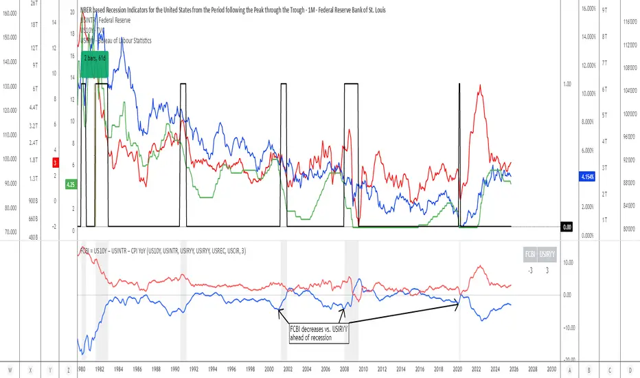
FCBI Brake PressureBrake Pressure (FCBI − USIRYY)
Concept
The Brake Pressure indicator quantifies whether the bond market is braking or releasing liquidity relative to real yields (USIRYY).
It is derived from the Financial-Conditions Brake Index (FCBI) and expresses the balance between long-term yield pressure and real-rate dynamics.
Formula
Brake Pressure = FCBI − USIRYY
where FCBI = (US10Y) − (USINTR) − (CPI YoY)
Purpose
While FCBI measures the intensity of financial-condition pressure, Brake Pressure shows when that brake is being applied or released.
It captures the turning point of liquidity transmission in the financial system.
How to Read
Brake Pressure < 0 (orange) → Brake engaged → financial conditions tighter than real-rate baseline; liquidity constrained.
Brake Pressure ≈ 0 → Neutral zone → transition phase between tightening and easing.
Brake Pressure > 0 (teal) → Brake released → financial conditions looser than real-rate baseline; liquidity flows freely → late-cycle setup before recession.
Zero-Cross Logic
Cross ↑ above 0 → FCBI > USIRYY → brake released → liquidity acceleration → typically 6–18 months before recession.
Cross ↓ below 0 → FCBI < USIRYY → brake re-engaged → tightening resumes.
Historical Behavior
Each major U.S. recession (2001, 2008, 2020) was preceded by a Brake Pressure cross above zero after a negative phase, signaling that long yields had stopped resisting Fed cuts and liquidity was expanding.
Practical Use
• Identify late-cycle turning points and liquidity inflection phases.
• Combine with FCBI for a complete macro transmission picture.
• Watch for sustained positive readings as early macro-recession warnings.
Current Example (Oct 2025)
FCBI ≈ −3.1, USIRYY ≈ +3.0 → Brake Pressure ≈ −6.1 → Brake still engaged. When this crosses above 0, it signals that liquidity is free flowing and the recession countdown has begun.
Summary
FCBI shows how tight the brake is. Brake Pressure shows when the brake releases.
When Brake Pressure > 0, the system has entered the liquidity-expansion phase that historically precedes a U.S. recession.
Ehlers Ultrasmooth Filter (USF)# USF: Ultrasmooth Filter
## Overview and Purpose
The Ultrasmooth Filter (USF) is an advanced signal processing tool that represents the pinnacle of noise reduction technology for financial time series. Developed by John Ehlers, this filter implements a complex algorithm that provides exceptional smoothing capabilities while minimizing the lag typically associated with heavy filtering. USF builds upon the Super Smooth Filter (SSF) with enhanced noise suppression characteristics, making it particularly valuable for identifying clear trends in extremely noisy market conditions where even traditional smoothing techniques struggle to produce clean signals.
## Core Concepts
* **Maximum noise suppression:** Provides the highest level of noise reduction among Ehlers' filter designs
* **Optimized coefficient structure:** Uses carefully designed mathematical relationships to achieve superior filtering performance
* **Market application:** Particularly effective for long-term trend identification and minimizing false signals in highly volatile market conditions
The core innovation of USF is its second-order filter structure with optimized coefficients that create an exceptionally smooth frequency response. By careful mathematical design, USF achieves near-optimal noise suppression characteristics while minimizing the lag and waveform distortion that typically accompany such heavy filtering. This makes it especially valuable for identifying major market trends amid significant short-term volatility.
## Common Settings and Parameters
| Parameter | Default | Function | When to Adjust |
|-----------|---------|----------|---------------|
| Length | 20 | Controls the cutoff period | Increase for smoother signals, decrease for more responsiveness |
| Source | close | Price data used for calculation | Consider using hlc3 for a more balanced price representation |
**Pro Tip:** USF is ideal for defining major market trends - try using it with a length of 40-60 on daily charts to identify dominant market direction and ignoring shorter-term noise completely.
## Calculation and Mathematical Foundation
**Simplified explanation:**
The Ultrasmooth Filter creates an extremely clean price representation by combining current and past price data with previous filter outputs using precisely calculated mathematical relationships. This creates a highly effective "averaging" process that removes virtually all market noise while still maintaining the essential trend information.
**Technical formula:**
USF = (1-c1)X + (2c1-c2)X₁ - (c1+c3)X₂ + c2×USF₁ + c3×USF₂
Where coefficients are calculated as:
- a1 = exp(-1.414π/length)
- b1 = 2a1 × cos(1.414 × 180/length)
- c1 = (1 + c2 - c3)/4
- c2 = b1
- c3 = -a1²
> 🔍 **Technical Note:** The filter combines both feed-forward (X terms) and feedback (USF terms) components in a second-order structure, creating a response with exceptional roll-off characteristics and minimal passband ripple.
## Interpretation Details
The Ultrasmooth Filter can be used in various trading strategies:
* **Major trend identification:** The direction of USF indicates the dominant market trend with minimal noise interference
* **Signal generation:** Crossovers between price and USF generate high-reliability trade signals with minimal false positives
* **Support/resistance levels:** USF can act as strong dynamic support during uptrends and resistance during downtrends
* **Market regime identification:** The slope of USF helps identify whether markets are in trending or consolidation phases
* **Multiple timeframe analysis:** Using USF across different chart timeframes creates a cohesive picture of nested trend structures
## Limitations and Considerations
* **Significant lag:** The extreme smoothing comes with increased lag compared to lighter filters
* **Initialization period:** Requires more bars than simpler filters to stabilize at the start of data
* **Less suitable for short-term trading:** Generally too slow-responding for short-term strategies
* **Parameter sensitivity:** Performance depends on appropriate length selection for the timeframe
* **Complementary tools:** Best used alongside faster-responding indicators for timing signals
## References
* Ehlers, J.F. "Cycle Analytics for Traders," Wiley, 2013
* Ehlers, J.F. "Rocket Science for Traders," Wiley, 2001

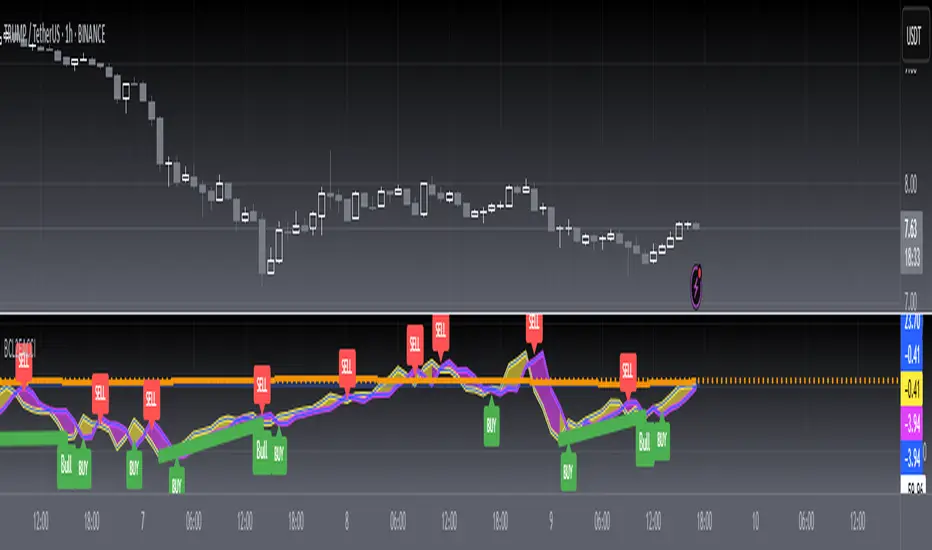
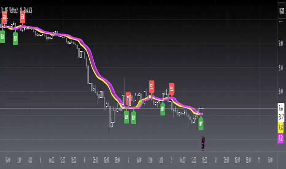
Buy/Sell Signals [WynTrader]My name is WynTrader. I cumulate 24 years of experience.
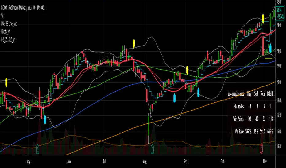
This Indicator produces Buy/Sell Signals using these features:
- Fast and Slow Moving averages (modifiable) optimized at EMA-8 and SMA-35
- Bollinger Bands (modifiable) optimized at Basis-18 and Multiplier-1
Also, the Buy/Sell Signals are conditioned by three Filters (optionable, modifiable) :
. Bollinger-Bands Lookback
. High-Low vs Candle Range %
. Distance from Fast and Slow Moving averages %
The Results Calculation presented in a Table are based :
- on the Current Chart Visible Range (optionable)
or
- on the specified TIme Frame Start and End Dates (modifiable)
The Table shows Calculation Results of the Buy and Sell Signals that are activated on the chart, with the Number of Trades (Signals), the Winning Points and the Win Rate %. The Buy&Hold starts calculation at the first Buy encountered.
So be surprised by my Buy/Sell Indicator. But always remember that the world is not perfect. The Graal Indicator, even with AI, doesn't already exist, maybe one day (all of us richier...), but not now. , depending on the chart product (stocks...), volatility, probabilities, unpredictable behaviour. , the moves, etc.
Enjoy
WynTrader
P. s. :
My name is WynTrader. I cumulate 24 years of experience. In 2001, I took an intensive technical analysis course taught by an exceptional friend, Cyril, who taught me everything I know. The foundation I gained through his teaching remains solid and relevant to this day, never failing me.
Before i made this Indicator, I have used many Trading View Buy/Sell Indicators using alone or combined RSI, SMI, OBV, MACD ATR, ADX, Neural, Fractal, Geometry, etc., that are already available for the Trading View community. A great thanks to those who give their time that help me build this tool.
Note that I'm not a programmer, so... ;-)
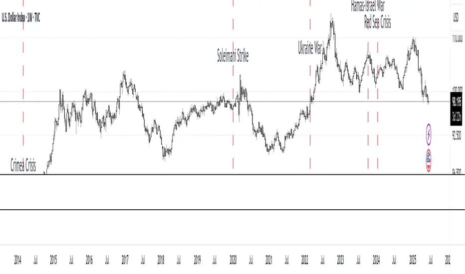
MC Geopolitical Tension Events📌 Script Title: Geopolitical Tension Events
📖 Description:
This script highlights key geopolitical and military tension events from 1914 to 2024 that have historically impacted global markets.
It automatically plots vertical dashed lines and labels on the chart at the time of each major event. This allows traders and analysts to visually assess how markets have responded to global crises, wars, and significant political instability over time.
🧠 Use Cases:
Historical backtesting: Understand how market responded to past geopolitical shocks.
Contextual analysis: Add macro context to technical setups.
🗓️ List of Geopolitical Tension Events in the Script
Date Event Title Description
1914-07-28 WWI Begins Outbreak of World War I following the assassination of Archduke Franz Ferdinand.
1929-10-24 Wall Street Crash Black Thursday, the start of the 1929 stock market crash.
1939-09-01 WWII Begins Germany invades Poland, starting World War II.
1941-12-07 Pearl Harbor Japanese attack on Pearl Harbor; U.S. enters WWII.
1945-08-06 Hiroshima Bombing First atomic bomb dropped on Hiroshima by the U.S.
1950-06-25 Korean War Begins North Korea invades South Korea.
1962-10-16 Cuban Missile Crisis 13-day standoff between the U.S. and USSR over missiles in Cuba.
1973-10-06 Yom Kippur War Egypt and Syria launch surprise attack on Israel.
1979-11-04 Iran Hostage Crisis U.S. Embassy in Tehran seized; 52 hostages taken.
1990-08-02 Gulf War Begins Iraq invades Kuwait, triggering U.S. intervention.
2001-09-11 9/11 Attacks Coordinated terrorist attacks on the U.S.
2003-03-20 Iraq War Begins U.S.-led invasion of Iraq to remove Saddam Hussein.
2008-09-15 Lehman Collapse Bankruptcy of Lehman Brothers; peak of global financial crisis.
2014-03-01 Crimea Crisis Russia annexes Crimea from Ukraine.
2020-01-03 Soleimani Strike U.S. drone strike kills Iranian General Qasem Soleimani.
2022-02-24 Ukraine Invasion Russia launches full-scale invasion of Ukraine.
2023-10-07 Hamas-Israel War Hamas launches attack on Israel, sparking war in Gaza.
2024-01-12 Red Sea Crisis Houthis attack ships in Red Sea, prompting Western naval response.
Bear Market Probability Model# Bear Market Probability Model: A Multi-Factor Risk Assessment Framework
The Bear Market Probability Model represents a comprehensive quantitative framework for assessing systemic market risk through the integration of 13 distinct risk factors across four analytical categories: macroeconomic indicators, technical analysis factors, market sentiment measures, and market breadth metrics. This indicator synthesizes established financial research methodologies to provide real-time probabilistic assessments of impending bear market conditions, offering institutional-grade risk management capabilities to retail and professional traders alike.
## Theoretical Foundation
### Historical Context of Bear Market Prediction
Bear market prediction has been a central focus of financial research since the seminal work of Dow (1901) and the subsequent development of technical analysis theory. The challenge of predicting market downturns gained renewed academic attention following the market crashes of 1929, 1987, 2000, and 2008, leading to the development of sophisticated multi-factor models.
Fama and French (1989) demonstrated that certain financial variables possess predictive power for stock returns, particularly during market stress periods. Their three-factor model laid the groundwork for multi-dimensional risk assessment, which this indicator extends through the incorporation of real-time market microstructure data.
### Methodological Framework
The model employs a weighted composite scoring methodology based on the theoretical framework established by Campbell and Shiller (1998) for market valuation assessment, extended through the incorporation of high-frequency sentiment and technical indicators as proposed by Baker and Wurgler (2006) in their seminal work on investor sentiment.
The mathematical foundation follows the general form:
Bear Market Probability = Σ(Wi × Ci) / ΣWi × 100
Where:
- Wi = Category weight (i = 1,2,3,4)
- Ci = Normalized category score
- Categories: Macroeconomic, Technical, Sentiment, Breadth
## Component Analysis
### 1. Macroeconomic Risk Factors
#### Yield Curve Analysis
The inclusion of yield curve inversion as a primary predictor follows extensive research by Estrella and Mishkin (1998), who demonstrated that the term spread between 3-month and 10-year Treasury securities has historically preceded all major recessions since 1969. The model incorporates both the 2Y-10Y and 3M-10Y spreads to capture different aspects of monetary policy expectations.
Implementation:
- 2Y-10Y Spread: Captures market expectations of monetary policy trajectory
- 3M-10Y Spread: Traditional recession predictor with 12-18 month lead time
Scientific Basis: Harvey (1988) and subsequent research by Ang, Piazzesi, and Wei (2006) established the theoretical foundation linking yield curve inversions to economic contractions through the expectations hypothesis of the term structure.
#### Credit Risk Premium Assessment
High-yield credit spreads serve as a real-time gauge of systemic risk, following the methodology established by Gilchrist and Zakrajšek (2012) in their excess bond premium research. The model incorporates the ICE BofA High Yield Master II Option-Adjusted Spread as a proxy for credit market stress.
Threshold Calibration:
- Normal conditions: < 350 basis points
- Elevated risk: 350-500 basis points
- Severe stress: > 500 basis points
#### Currency and Commodity Stress Indicators
The US Dollar Index (DXY) momentum serves as a risk-off indicator, while the Gold-to-Oil ratio captures commodity market stress dynamics. This approach follows the methodology of Akram (2009) and Beckmann, Berger, and Czudaj (2015) in analyzing commodity-currency relationships during market stress.
### 2. Technical Analysis Factors
#### Multi-Timeframe Moving Average Analysis
The technical component incorporates the well-established moving average convergence methodology, drawing from the work of Brock, Lakonishok, and LeBaron (1992), who provided empirical evidence for the profitability of technical trading rules.
Implementation:
- Price relative to 50-day and 200-day simple moving averages
- Moving average convergence/divergence analysis
- Multi-timeframe MACD assessment (daily and weekly)
#### Momentum and Volatility Analysis
The model integrates Relative Strength Index (RSI) analysis following Wilder's (1978) original methodology, combined with maximum drawdown analysis based on the work of Magdon-Ismail and Atiya (2004) on optimal drawdown measurement.
### 3. Market Sentiment Factors
#### Volatility Index Analysis
The VIX component follows the established research of Whaley (2009) and subsequent work by Bekaert and Hoerova (2014) on VIX as a predictor of market stress. The model incorporates both absolute VIX levels and relative VIX spikes compared to the 20-day moving average.
Calibration:
- Low volatility: VIX < 20
- Elevated concern: VIX 20-25
- High fear: VIX > 25
- Panic conditions: VIX > 30
#### Put-Call Ratio Analysis
Options flow analysis through put-call ratios provides insight into sophisticated investor positioning, following the methodology established by Pan and Poteshman (2006) in their analysis of informed trading in options markets.
### 4. Market Breadth Factors
#### Advance-Decline Analysis
Market breadth assessment follows the classic work of Fosback (1976) and subsequent research by Brown and Cliff (2004) on market breadth as a predictor of future returns.
Components:
- Daily advance-decline ratio
- Advance-decline line momentum
- McClellan Oscillator (Ema19 - Ema39 of A-D difference)
#### New Highs-New Lows Analysis
The new highs-new lows ratio serves as a market leadership indicator, based on the research of Zweig (1986) and validated in academic literature by Zarowin (1990).
## Dynamic Threshold Methodology
The model incorporates adaptive thresholds based on rolling volatility and trend analysis, following the methodology established by Pagan and Sossounov (2003) for business cycle dating. This approach allows the model to adjust sensitivity based on prevailing market conditions.
Dynamic Threshold Calculation:
- Warning Level: Base threshold ± (Volatility × 1.0)
- Danger Level: Base threshold ± (Volatility × 1.5)
- Bounds: ±10-20 points from base threshold
## Professional Implementation
### Institutional Usage Patterns
Professional risk managers typically employ multi-factor bear market models in several contexts:
#### 1. Portfolio Risk Management
- Tactical Asset Allocation: Reducing equity exposure when probability exceeds 60-70%
- Hedging Strategies: Implementing protective puts or VIX calls when warning thresholds are breached
- Sector Rotation: Shifting from growth to defensive sectors during elevated risk periods
#### 2. Risk Budgeting
- Value-at-Risk Adjustment: Incorporating bear market probability into VaR calculations
- Stress Testing: Using probability levels to calibrate stress test scenarios
- Capital Requirements: Adjusting regulatory capital based on systemic risk assessment
#### 3. Client Communication
- Risk Reporting: Quantifying market risk for client presentations
- Investment Committee Decisions: Providing objective risk metrics for strategic decisions
- Performance Attribution: Explaining defensive positioning during market stress
### Implementation Framework
Professional traders typically implement such models through:
#### Signal Hierarchy:
1. Probability < 30%: Normal risk positioning
2. Probability 30-50%: Increased hedging, reduced leverage
3. Probability 50-70%: Defensive positioning, cash building
4. Probability > 70%: Maximum defensive posture, short exposure consideration
#### Risk Management Integration:
- Position Sizing: Inverse relationship between probability and position size
- Stop-Loss Adjustment: Tighter stops during elevated risk periods
- Correlation Monitoring: Increased attention to cross-asset correlations
## Strengths and Advantages
### 1. Comprehensive Coverage
The model's primary strength lies in its multi-dimensional approach, avoiding the single-factor bias that has historically plagued market timing models. By incorporating macroeconomic, technical, sentiment, and breadth factors, the model provides robust risk assessment across different market regimes.
### 2. Dynamic Adaptability
The adaptive threshold mechanism allows the model to adjust sensitivity based on prevailing volatility conditions, reducing false signals during low-volatility periods and maintaining sensitivity during high-volatility regimes.
### 3. Real-Time Processing
Unlike traditional academic models that rely on monthly or quarterly data, this indicator processes daily market data, providing timely risk assessment for active portfolio management.
### 4. Transparency and Interpretability
The component-based structure allows users to understand which factors are driving risk assessment, enabling informed decision-making about model signals.
### 5. Historical Validation
Each component has been validated in academic literature, providing theoretical foundation for the model's predictive power.
## Limitations and Weaknesses
### 1. Data Dependencies
The model's effectiveness depends heavily on the availability and quality of real-time economic data. Federal Reserve Economic Data (FRED) updates may have lags that could impact model responsiveness during rapidly evolving market conditions.
### 2. Regime Change Sensitivity
Like most quantitative models, the indicator may struggle during unprecedented market conditions or structural regime changes where historical relationships break down (Taleb, 2007).
### 3. False Signal Risk
Multi-factor models inherently face the challenge of balancing sensitivity with specificity. The model may generate false positive signals during normal market volatility periods.
### 4. Currency and Geographic Bias
The model focuses primarily on US market indicators, potentially limiting its effectiveness for global portfolio management or non-USD denominated assets.
### 5. Correlation Breakdown
During extreme market stress, correlations between risk factors may increase dramatically, reducing the model's diversification benefits (Forbes and Rigobon, 2002).
## References
Akram, Q. F. (2009). Commodity prices, interest rates and the dollar. Energy Economics, 31(6), 838-851.
Ang, A., Piazzesi, M., & Wei, M. (2006). What does the yield curve tell us about GDP growth? Journal of Econometrics, 131(1-2), 359-403.
Baker, M., & Wurgler, J. (2006). Investor sentiment and the cross‐section of stock returns. The Journal of Finance, 61(4), 1645-1680.
Baker, S. R., Bloom, N., & Davis, S. J. (2016). Measuring economic policy uncertainty. The Quarterly Journal of Economics, 131(4), 1593-1636.
Barber, B. M., & Odean, T. (2001). Boys will be boys: Gender, overconfidence, and common stock investment. The Quarterly Journal of Economics, 116(1), 261-292.
Beckmann, J., Berger, T., & Czudaj, R. (2015). Does gold act as a hedge or a safe haven for stocks? A smooth transition approach. Economic Modelling, 48, 16-24.
Bekaert, G., & Hoerova, M. (2014). The VIX, the variance premium and stock market volatility. Journal of Econometrics, 183(2), 181-192.
Brock, W., Lakonishok, J., & LeBaron, B. (1992). Simple technical trading rules and the stochastic properties of stock returns. The Journal of Finance, 47(5), 1731-1764.
Brown, G. W., & Cliff, M. T. (2004). Investor sentiment and the near-term stock market. Journal of Empirical Finance, 11(1), 1-27.
Campbell, J. Y., & Shiller, R. J. (1998). Valuation ratios and the long-run stock market outlook. The Journal of Portfolio Management, 24(2), 11-26.
Dow, C. H. (1901). Scientific stock speculation. The Magazine of Wall Street.
Estrella, A., & Mishkin, F. S. (1998). Predicting US recessions: Financial variables as leading indicators. Review of Economics and Statistics, 80(1), 45-61.
Fama, E. F., & French, K. R. (1989). Business conditions and expected returns on stocks and bonds. Journal of Financial Economics, 25(1), 23-49.
Forbes, K. J., & Rigobon, R. (2002). No contagion, only interdependence: measuring stock market comovements. The Journal of Finance, 57(5), 2223-2261.
Fosback, N. G. (1976). Stock market logic: A sophisticated approach to profits on Wall Street. The Institute for Econometric Research.
Gilchrist, S., & Zakrajšek, E. (2012). Credit spreads and business cycle fluctuations. American Economic Review, 102(4), 1692-1720.
Harvey, C. R. (1988). The real term structure and consumption growth. Journal of Financial Economics, 22(2), 305-333.
Kahneman, D., & Tversky, A. (1979). Prospect theory: An analysis of decision under risk. Econometrica, 47(2), 263-291.
Magdon-Ismail, M., & Atiya, A. F. (2004). Maximum drawdown. Risk, 17(10), 99-102.
Nickerson, R. S. (1998). Confirmation bias: A ubiquitous phenomenon in many guises. Review of General Psychology, 2(2), 175-220.
Pagan, A. R., & Sossounov, K. A. (2003). A simple framework for analysing bull and bear markets. Journal of Applied Econometrics, 18(1), 23-46.
Pan, J., & Poteshman, A. M. (2006). The information in option volume for future stock prices. The Review of Financial Studies, 19(3), 871-908.
Taleb, N. N. (2007). The black swan: The impact of the highly improbable. Random House.
Whaley, R. E. (2009). Understanding the VIX. The Journal of Portfolio Management, 35(3), 98-105.
Wilder, J. W. (1978). New concepts in technical trading systems. Trend Research.
Zarowin, P. (1990). Size, seasonality, and stock market overreaction. Journal of Financial and Quantitative Analysis, 25(1), 113-125.
Zweig, M. E. (1986). Winning on Wall Street. Warner Books.

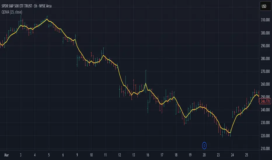
Quadruple EMA (QEMA)The Quadruple Exponential Moving Average (QEMA) is an advanced technical indicator that extends the concept of lag reduction beyond TEMA (Triple Exponential Moving Average) to a fourth order. By applying a sophisticated four-stage EMA cascade with optimized coefficient distribution, QEMA provides the ultimate evolution in EMA-based lag reduction techniques.
Unlike traditional compund moving averages like DEMA and TEMA, QEMA implements a progressive smoothing system that strategically distributes alphas across four EMA stages and combines them with balanced coefficients (4, -6, 4, -1). This approach creates an indicator that responds extremely quickly to price changes while still maintaining sufficient smoothness to be useful for trading decisions. QEMA is particularly valuable for traders who need the absolute minimum lag possible in trend identification.
▶️ **Core Concepts**
Fourth-order processing: Extends the EMA cascade to four stages for maximum possible lag reduction while maintaining a useful signal
Progressive alpha system: Uses mathematically derived ratio-based alpha progression to balance responsiveness across all four EMA stages
Optimized coefficients: Employs calculated weights (4, -6, 4, -1) to effectively eliminate lag while preserving compound signal stability
Numerical stability control: Implements initialization and alpha distribution to ensure consistent results from the first calculation bar
QEMA achieves its exceptional lag reduction by combining four progressive EMAs with mathematically optimized coefficients. The formula is designed to maximize responsiveness while minimizing the overshoot problems that typically occur with aggressive lag reduction techniques. The implementation uses a ratio-based alpha progression that ensures each EMA stage contributes appropriately to the final result.
▶️ **Common Settings and Parameters**
Period: Default: 15| Base smoothing period | When to Adjust: Decrease for extremely fast signals, increase for more stable output
Alpha: Default: auto | Direct control of base smoothing factor | When to Adjust: Manual setting allows precise tuning beyond standard period settings
Source: Default: Close | Data point used for calculation | When to Adjust: Change to HL2 or HLC3 for more balanced price representation
Pro Tip: Professional traders often use QEMA with longer periods than other moving averages (e.g., QEMA(20) instead of EMA(10)) since its extreme lag reduction provides earlier signals even with longer periods.
▶️ **Calculation and Mathematical Foundation**
Simplified explanation:
QEMA works by calculating four EMAs in sequence, with each EMA taking the previous one as input. It then combines these EMAs using balancing weights (4, -6, 4, -1) to create a moving average with extremely minimal lag and high level of smoothness. The alpha factors for each EMA are progressively adjusted using a mathematical ratio to ensure balanced responsiveness across all stages.
Technical formula:
QEMA = 4 × EMA₁ - 6 × EMA₂ + 4 × EMA₃ - EMA₄
Where:
EMA₁ = EMA(source, α₁)
EMA₂ = EMA(EMA₁, α₂)
EMA₃ = EMA(EMA₂, α₃)
EMA₄ = EMA(EMA₃, α₄)
α₁ = 2/(period + 1) is the base smoothing factor
r = (1/α₁)^(1/3) is the derived ratio
α₂ = α₁ × r, α₃ = α₂ × r, α₄ = α₃ × r are the progressive alphas
Mathematical Rationale for the Alpha Cascade:
The QEMA indicator employs a specific geometric progression for its smoothing factors (alphas) across the four EMA stages. This design is intentional and aims to optimize the filter's performance. The ratio between alphas is **r = (1/α₁)^(1/3)** - derived from the cube root of the reciprocal of the base alpha.
For typical smoothing (α₁ < 1), this results in a sequence of increasing alpha values (α₁ < α₂ < α₃ < α₄), meaning that subsequent EMAs in the cascade are progressively faster (less smoothed). This specific progression, when combined with the QEMA coefficients (4, -6, 4, -1), is chosen for the following reasons:
1. Optimized Frequency Response:
Using the same alpha for all EMA stages (as in a naive multi-EMA approach) can lead to an uneven frequency response, potentially causing over-shooting of certain frequencies or creating undesirable resonance. The geometric progression of alphas in QEMA helps to create a more balanced and controlled filter response across a wider range of movement frequencies. Each stage's contribution to the overall filtering characteristic is more harmonized.
2. Minimized Phase Lag:
A key goal of QEMA is extreme lag reduction. The specific alpha cascade, particularly the relationship defined by **r**, is designed to minimize the cumulative phase lag introduced by the four smoothing stages, while still providing effective noise reduction. Faster subsequent EMAs contribute to this reduced lag.
🔍 Technical Note: The ratio-based alpha progression is crucial for balanced response. The ratio r is calculated as the cube root of 1/α₁, ensuring that the combined effect of all four EMAs creates a mathematically optimal response curve. All EMAs are initialized with the first source value rather than using progressive initialization, eliminating warm-up artifacts and providing consistent results from the first bar.
▶️ **Interpretation Details**
QEMA provides several key insights for traders:
When price crosses above QEMA, it signals the beginning of an uptrend with minimal delay
When price crosses below QEMA, it signals the beginning of a downtrend with minimal delay
The slope of QEMA provides immediate insight into trend direction and momentum
QEMA responds to price reversals significantly faster than other moving averages
Multiple QEMA lines with different periods can identify immediate support/resistance levels
QEMA is particularly valuable in fast-moving markets and for short-term trading strategies where speed of signal generation is critical. It excels at capturing the very beginning of trends and identifying reversals earlier than any other EMA-derived indicator. This makes it especially useful for breakout trading and scalping strategies where getting in early is essential.
▶️ **Limitations and Considerations**
Market conditions: Can generate excessive signals in choppy, sideways markets due to its extreme responsiveness
Overshooting: The aggressive lag reduction can create some overshooting during sharp reversals
Calculation complexity: Requires four separate EMA calculations plus coefficient application, making it computationally more intensive
Parameter sensitivity: Small changes in the base alpha or period can significantly alter behavior
Complementary tools: Should be used with momentum indicators or volatility filters to confirm signals and reduce false positives
▶️ **References**
Mulloy, P. (1994). "Smoothing Data with Less Lag," Technical Analysis of Stocks & Commodities .
Ehlers, J. (2001). Rocket Science for Traders . John Wiley & Sons.
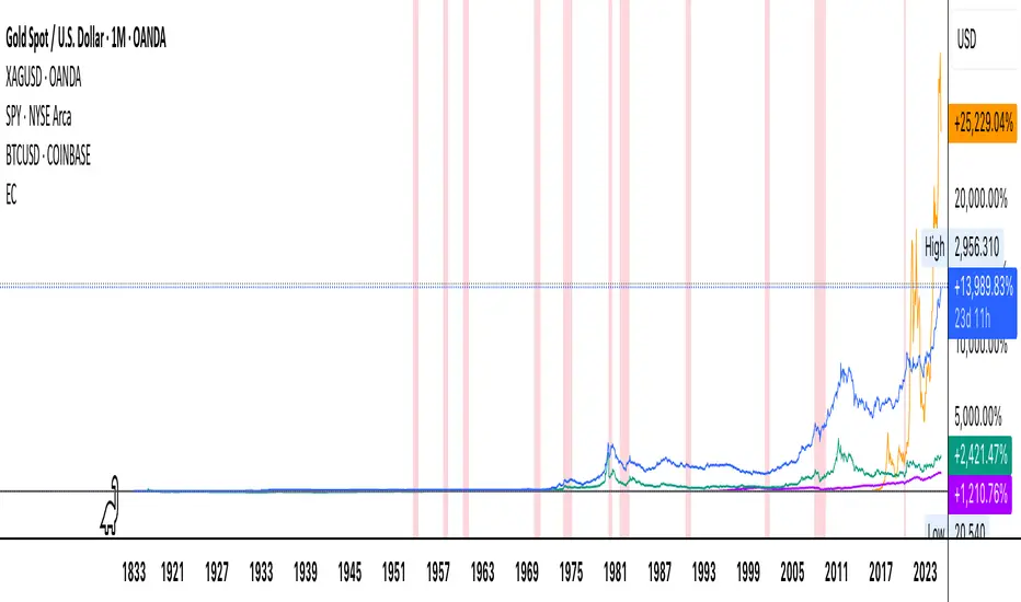
Economic Crises by @zeusbottradingEconomic Crises Indicator by @zeusbottrading
Description and Use Case
Overview
The Economic Crises Highlight Indicator is designed to visually mark major economic crises on a TradingView chart by shading these periods in red. It provides a historical context for financial analysis by indicating when major recessions occurred, helping traders and analysts assess the performance of assets before, during, and after these crises.
What This Indicator Shows
This indicator highlights the following major economic crises (from 1953 to 2020), which significantly impacted global markets:
• 1953 Korean War Recession
• 1957 Monetary Tightening Recession
• 1960 Investment Decline Recession
• 1969 Employment Crisis
• 1973 Oil Crisis
• 1980 Inflation Crisis
• 1981 Fed Monetary Policy Recession
• 1990 Oil Crisis and Gulf War Recession
• 2001 Dot-Com Bubble Crash
• 2008 Global Financial Crisis (Great Recession)
• 2020 COVID-19 Recession
Each of these periods is shaded in red with 80% transparency, allowing you to clearly see the impact of economic downturns on various financial assets.
How This Indicator is Useful
This indicator is particularly valuable for:
✅ Comparative Performance Analysis – It allows traders and investors to compare how different assets (e.g., Gold, Silver, S&P 500, Bitcoin) performed before, during, and after major economic crises.
✅ Identifying Market Trends – Helps recognize recurring patterns in asset price movements during times of financial distress.
✅ Risk Management & Strategy Development – Understanding how markets reacted in the past can assist in making better-informed investment decisions for future downturns.
✅ Gold, Silver & Bitcoin as Safe Havens – Comparing precious metals and cryptocurrencies against traditional stocks (e.g., SPY) to analyze their performance as hedges during economic turmoil.
How to Use It in Your Analysis
By overlaying this indicator on your Gold, Silver, SPY, and Bitcoin chart (for example), you can quickly spot historical market reactions and use that insight to predict possible behaviors in future downturns.
⸻
How to Apply This in TradingView?
1. Click on Use on chart under the image.
2. Overlay it with Gold ( OANDA:XAUUSD ), Silver ( OANDA:XAGUSD ), SPY ( AMEX:SPY ), and Bitcoin ( COINBASE:BTCUSD ) for comparative analysis.
⸻
Conclusion
This indicator serves as a powerful historical reference for traders analyzing asset performance during economic downturns. By studying past crises, you can develop a data-driven investment strategy and improve your market insights. 🚀📈
Let me know if you need any modifications or enhancements!
Temporary Help Services Jobs - Trend Allocation StrategyThis strategy is designed to capitalize on the economic trends represented by the Temporary Help Services (TEMPHELPS) index, which is published by the Federal Reserve Economic Data (FRED). Temporary Help Services Jobs are often regarded as a leading indicator of labor market conditions, as changes in temporary employment levels frequently precede broader employment trends.
Methodology:
Data Source: The strategy uses the FRED dataset TEMPHELPS for monthly data on temporary help services.
Trend Definition:
Uptrend: When the current month's value is greater than the previous month's value.
Downtrend: When the current month's value is less than the previous month's value.
Entry Condition: A long position is opened when an uptrend is detected, provided no position is currently held.
Exit Condition: The long position is closed when a downtrend is detected.
Scientific Basis:
The TEMPHELPS index serves as a leading economic indicator, as noted in studies analyzing labor market cyclicality (e.g., Katz & Krueger, 1999). Temporary employment is often considered a proxy for broader economic conditions, particularly in predicting recessions or recoveries. Incorporating this index into trading strategies allows for aligning trades with potential macroeconomic shifts, as suggested by research on employment trends and market performance (Autor, 2001; Valetta & Bengali, 2013).
Usage:
This strategy is best suited for long-term investors or macroeconomic trend followers who wish to leverage labor market signals for equity or futures trading. It operates exclusively on end-of-month data, ensuring minimal transaction costs and noise.

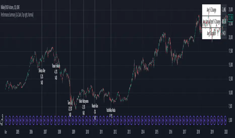
Performance Summary and Shading (Offset Version)Modified "Recession and Crisis Shading" Indicator by @haribotagada (Original Link: )
The updated indicator accepts a days offset (positive or negative) to calculate performance between the offset date and the input date.
Potential uses include identifying performance one week after company earnings or an FOMC meeting.
This feature simplifies input by enabling standardized offset dates, while still allowing flexibility to adjust ranges by overriding inputs as needed.
Summary of added features and indicator notes:
Inputs both positive and negative offset.
By default, the script calculates performance from the close of the input date to the close of the date at (input date + offset) for positive offsets, and from the close of (input date - offset) to the close of the input date for negative offsets. For example, with an input date of November 1, 2024, an offset of 7 calculates performance from the close on November 1 to the close on November 8, while an offset of -7 calculates from the close on October 25 to the close on November 1.
Allows user to perform the calculation using the open price on the input date instead of close price
The input format has been modified to allow overrides for the default duration, while retaining the original capabilities of the indicator.
The calculation shows both the average change and the average annualized change. For bar-wise calculations, annualization assumes 252 trading days per year. For date-wise calculations, it assumes 365 days for annualization.
Carries over all previous inputs to retain functionality of the previous script. Changes a few small settings:
Calculates start to end date performance by default instead of peak to trough performance.
Updates visuals of label text to make it easier to read and less transparent.
Changed stat box color scheme to make the text easier to read
Updated default input data to new format of input with offsets
Changed default duration statistic to number of days instead of number of bars with an option to select number of bars.
Potential Features to Add:
Import dataset from CSV files or by plugging into TradingView calendar
Example Input Datasets:
Recessions:
2020-02-01,COVID-19,59
2007-12-01,Subprime mortgages,547
2001-03-01,Dot-com,243
1990-07-01,Oil shock,243
1981-07-01,US unemployment,788
1980-01-01,Volker,182
1973-11-01,OPEC,485
Japan Revolving Door Elections
2006-09-26, Shinzo Abe
2007-09-26, Yasuo Fukuda
2008-09-24, Taro Aso
2009-09-16, Yukio Hatoyama
2010-07-08, Naoto Kan
2011-09-02, Yoshihiko Noda
Hope you find the modified indicator useful and let me know if you would like any features to be added!
Currency Futures StatisticsThe "Currency Futures Statistics" indicator provides comprehensive insights into the performance and characteristics of various currency futures. This indicator is crucial for portfolio management as it combines multiple metrics that are instrumental in evaluating currency futures' risk and return profiles.
Metrics Included:
Historical Volatility:
Definition: Historical volatility measures the standard deviation of returns over a specified period, scaled to an annual basis.
Importance: High volatility indicates greater price fluctuations, which translates to higher risk. Investors and portfolio managers use volatility to gauge the stability of a currency future and to make informed decisions about risk management and position sizing (Hull, J. C. (2017). Options, Futures, and Other Derivatives).
Open Interest:
Definition: Open interest represents the total number of outstanding futures contracts that are held by market participants.
Importance: High open interest often signifies liquidity in the market, meaning that entering and exiting positions is less likely to impact the price significantly. It also reflects market sentiment and the degree of participation in the futures market (Black, F., & Scholes, M. (1973). The Pricing of Options and Corporate Liabilities).
Year-over-Year (YoY) Performance:
Definition: YoY performance calculates the percentage change in the futures contract's price compared to the same week from the previous year.
Importance: This metric provides insight into the long-term trend and relative performance of a currency future. Positive YoY performance suggests strengthening trends, while negative values indicate weakening trends (Fama, E. F. (1991). Efficient Capital Markets: II).
200-Day Simple Moving Average (SMA) Position:
Definition: This metric indicates whether the current price of the currency future is above or below its 200-day simple moving average.
Importance: The 200-day SMA is a widely used trend indicator. If the price is above the SMA, it suggests a bullish trend, while being below indicates a bearish trend. This information is vital for trend-following strategies and can help in making buy or sell decisions (Bollinger, J. (2001). Bollinger on Bollinger Bands).
Why These Metrics are Important for Portfolio Management:
Risk Assessment: Historical volatility and open interest provide essential information for assessing the risk associated with currency futures. Understanding the volatility helps in estimating potential price swings, which is crucial for managing risk and setting appropriate stop-loss levels.
Liquidity and Market Participation: Open interest is a critical indicator of market liquidity. Higher open interest usually means tighter bid-ask spreads and better liquidity, which facilitates smoother trading and better execution of trades.
Trend Analysis: YoY performance and the SMA position help in analyzing long-term trends. This analysis is crucial for making strategic investment decisions and adjusting the portfolio based on changing market conditions.
Informed Decision-Making: Combining these metrics allows for a holistic view of the currency futures market. This comprehensive view helps in making informed decisions, balancing risks and returns, and optimizing the portfolio to align with investment goals.
In summary, the "Currency Futures Statistics" indicator equips investors and portfolio managers with valuable data points that are essential for effective risk management, liquidity assessment, trend analysis, and overall portfolio optimization.

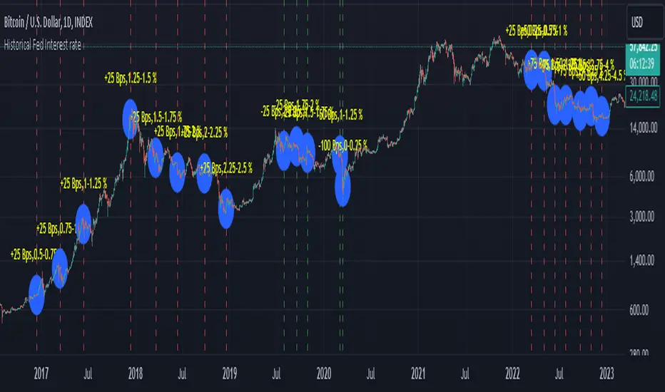
Historical Fed Interest rate This script is Historical Fed Interest rate
The data is between 1991 - 2023 , but for some reason data between 1991 - 10/2001 is not work
Green line for rate cut and Red line for rate hike and detail at the label
Month/Month Percentage % Change, Historical; Seasonal TendencyTable of monthly % changes in Average Price over the last 10 years (or the 10 yrs prior to input year).
Useful for gauging seasonal tendencies of an asset; backtesting monthly volatility and bullish/bearish tendency.
~~User Inputs~~
Choose measure of average: sma(close), sma(ohlc4), vwap(close), vwma(close).
Show last 10yrs, with 10yr average % change, or to just show single year.
Chose input year; with the indicator auto calculating the prior 10 years.
Choose color for labels and size for labels; choose +Ve value color and -Ve value color.
Set 'Daily bars in month': 21 for Forex/Commodities/Indices; 30 for Crypto.
Set precision: decimal places
~~notes~~
-designed for use on Daily timeframe (tradingview is buggy on monthly timeframe calculations, and less precise on weekly timeframe calculations).
-where Current month of year has not occurred yet, will print 9yr average.
-calculates the average change of displayed month compared to the previous month: i.e. Jan22 value represents whole of Jan22 compared to whole of Dec21.
-table displays on the chart over the input year; so for ES, with 2010 selected; shows values from 2001-2010, displaying across 2010-2011 on the chart.
-plots on seperate right hand side scale, so can be shrunk and dragged vertically.
-thanks to @gabx11 for the suggestion which inspired me to write this

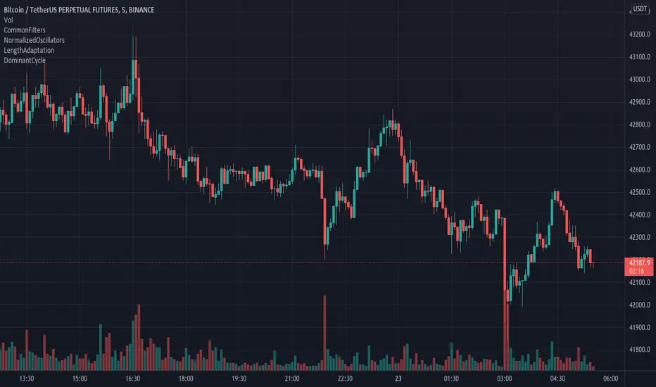
DominantCycleCollection of Dominant Cycle estimators. Length adaptation used in the Adaptive Moving Averages and the Adaptive Oscillators try to follow price movements and accelerate/decelerate accordingly (usually quite rapidly with a huge range). Cycle estimators, on the other hand, try to measure the cycle period of the current market, which does not reflect price movement or the rate of change (the rate of change may also differ depending on the cycle phase, but the cycle period itself usually changes slowly). This collection may become encyclopaedic, so if you have any working cycle estimator, drop me a line in the comments below. Suggestions are welcome. Currently included estimators are based on the work of John F. Ehlers
mamaPeriod(src, dynLow, dynHigh) MESA Adaptation - MAMA Cycle
Parameters:
src : Series to use
dynLow : Lower bound for the dynamic length
dynHigh : Upper bound for the dynamic length
Returns: Calculated period
Based on MESA Adaptive Moving Average by John F. Ehlers
Performs Hilbert Transform Homodyne Discriminator cycle measurement
Unlike MAMA Alpha function (in LengthAdaptation library), this does not compute phase rate of change
Introduced in the September 2001 issue of Stocks and Commodities
Inspired by the @everget implementation:
Inspired by the @anoojpatel implementation:
paPeriod(src, dynLow, dynHigh, preHP, preSS, preHP) Pearson Autocorrelation
Parameters:
src : Series to use
dynLow : Lower bound for the dynamic length
dynHigh : Upper bound for the dynamic length
preHP : Use High Pass prefilter (default)
preSS : Use Super Smoother prefilter (default)
preHP : Use Hann Windowing prefilter
Returns: Calculated period
Based on Pearson Autocorrelation Periodogram by John F. Ehlers
Introduced in the September 2016 issue of Stocks and Commodities
Inspired by the @blackcat1402 implementation:
Inspired by the @rumpypumpydumpy implementation:
Corrected many errors, and made small speed optimizations, so this could be the best implementation to date (still slow, though, so may revisit in future)
High Pass and Super Smoother prefilters are used in the original implementation
dftPeriod(src, dynLow, dynHigh, preHP, preSS, preHP) Discrete Fourier Transform
Parameters:
src : Series to use
dynLow : Lower bound for the dynamic length
dynHigh : Upper bound for the dynamic length
preHP : Use High Pass prefilter (default)
preSS : Use Super Smoother prefilter (default)
preHP : Use Hann Windowing prefilter
Returns: Calculated period
Based on Spectrum from Discrete Fourier Transform by John F. Ehlers
Inspired by the @blackcat1402 implementation:
High Pass, Super Smoother and Hann Windowing prefilters are used in the original implementation
phasePeriod(src, dynLow, dynHigh, preHP, preSS, preHP) Phase Accumulation
Parameters:
src : Series to use
dynLow : Lower bound for the dynamic length
dynHigh : Upper bound for the dynamic length
preHP : Use High Pass prefilter (default)
preSS : Use Super Smoother prefilter (default)
preHP : Use Hamm Windowing prefilter
Returns: Calculated period
Based on Dominant Cycle from Phase Accumulation by John F. Ehlers
High Pass and Super Smoother prefilters are used in the original implementation
doAdapt(type, src, len, dynLow, dynHigh, chandeSDLen, chandeSmooth, chandePower, preHP, preSS, preHP) Execute a particular Length Adaptation or Dominant Cycle Estimator from the list
Parameters:
type : Length Adaptation or Dominant Cycle Estimator type to use
src : Series to use
len : Reference lookback length
dynLow : Lower bound for the dynamic length
dynHigh : Upper bound for the dynamic length
chandeSDLen : Lookback length of Standard deviation for Chande's Dynamic Length
chandeSmooth : Smoothing length of Standard deviation for Chande's Dynamic Length
chandePower : Exponent of the length adaptation for Chande's Dynamic Length (lower is smaller variation)
preHP : Use High Pass prefilter for the Estimators that support it (default)
preSS : Use Super Smoother prefilter for the Estimators that support it (default)
preHP : Use Hann Windowing prefilter for the Estimators that support it
Returns: Calculated period (float, not limited)
doEstimate(type, src, dynLow, dynHigh, preHP, preSS, preHP) Execute a particular Dominant Cycle Estimator from the list
Parameters:
type : Dominant Cycle Estimator type to use
src : Series to use
dynLow : Lower bound for the dynamic length
dynHigh : Upper bound for the dynamic length
preHP : Use High Pass prefilter for the Estimators that support it (default)
preSS : Use Super Smoother prefilter for the Estimators that support it (default)
preHP : Use Hann Windowing prefilter for the Estimators that support it
Returns: Calculated period (float, not limited)
LengthAdaptationCollection of dynamic length adaptation algorithms. Mostly from various Adaptive Moving Averages (they are usually just EMA otherwise). Now you can combine Adaptations with any other Moving Averages or Oscillators (see my other libraries), to get something like Deviation Scaled RSI or Fractal Adaptive VWMA. This collection is not encyclopaedic. Suggestions are welcome.
chande(src, len, sdlen, smooth, power) Chande's Dynamic Length
Parameters:
src : Series to use
len : Reference lookback length
sdlen : Lookback length of Standard deviation
smooth : Smoothing length of Standard deviation
power : Exponent of the length adaptation (lower is smaller variation)
Returns: Calculated period
Taken from Chande's Dynamic Momentum Index (CDMI or DYMOI), which is dynamic RSI with this length
Original default power value is 1, but I use 0.5
A variant of this algorithm is also included, where volume is used instead of price
vidya(src, len, dynLow) Variable Index Dynamic Average Indicator (VIDYA)
Parameters:
src : Series to use
len : Reference lookback length
dynLow : Lower bound for the dynamic length
Returns: Calculated period
Standard VIDYA algorithm. The period oscillates from the Lower Bound up (slow)
I took the adaptation part, as it is just an EMA otherwise
vidyaRS(src, len, dynHigh) Relative Strength Dynamic Length - VIDYA RS
Parameters:
src : Series to use
len : Reference lookback length
dynHigh : Upper bound for the dynamic length
Returns: Calculated period
Based on Vitali Apirine's modification (Stocks and Commodities, January 2022) of VIDYA algorithm. The period oscillates from the Upper Bound down (fast)
I took the adaptation part, as it is just an EMA otherwise
kaufman(src, len, dynLow, dynHigh) Kaufman Efficiency Scaling
Parameters:
src : Series to use
len : Reference lookback length
dynLow : Lower bound for the dynamic length
dynHigh : Upper bound for the dynamic length
Returns: Calculated period
Based on Efficiency Ratio calculation orifinally used in Kaufman Adaptive Moving Average developed by Perry J. Kaufman
I took the adaptation part, as it is just an EMA otherwise
ds(src, len) Deviation Scaling
Parameters:
src : Series to use
len : Reference lookback length
Returns: Calculated period
Based on Derivation Scaled Super Smoother (DSSS) by John F. Ehlers
Originally used with Super Smoother
RMS originally has 50 bar lookback. Changed to 4x length for better flexibility. Could be wrong.
maa(src, len, threshold) Median Average Adaptation
Parameters:
src : Series to use
len : Reference lookback length
threshold : Adjustment threshold (lower is smaller length, default: 0.002, min: 0.0001)
Returns: Calculated period
Based on Median Average Adaptive Filter by John F. Ehlers
Discovered and implemented by @cheatcountry:
I took the adaptation part, as it is just an EMA otherwise
fra(len, fc, sc) Fractal Adaptation
Parameters:
len : Reference lookback length
fc : Fast constant (default: 1)
sc : Slow constant (default: 200)
Returns: Calculated period
Based on FRAMA by John F. Ehlers
Modified to allow lower and upper bounds by an unknown author
I took the adaptation part, as it is just an EMA otherwise
mama(src, dynLow, dynHigh) MESA Adaptation - MAMA Alpha
Parameters:
src : Series to use
dynLow : Lower bound for the dynamic length
dynHigh : Upper bound for the dynamic length
Returns: Calculated period
Based on MESA Adaptive Moving Average by John F. Ehlers
Introduced in the September 2001 issue of Stocks and Commodities
Inspired by the @everget implementation:
I took the adaptation part, as it is just an EMA otherwise
doAdapt(type, src, len, dynLow, dynHigh, chandeSDLen, chandeSmooth, chandePower) Execute a particular Length Adaptation from the list
Parameters:
type : Length Adaptation type to use
src : Series to use
len : Reference lookback length
dynLow : Lower bound for the dynamic length
dynHigh : Upper bound for the dynamic length
chandeSDLen : Lookback length of Standard deviation for Chande's Dynamic Length
chandeSmooth : Smoothing length of Standard deviation for Chande's Dynamic Length
chandePower : Exponent of the length adaptation for Chande's Dynamic Length (lower is smaller variation)
Returns: Calculated period (float, not limited)
doMA(type, src, len) MA wrapper on wrapper: if DSSS is selected, calculate it here
Parameters:
type : MA type to use
src : Series to use
len : Filtering length
Returns: Filtered series
Demonstration of a combined indicator: Deviation Scaled Super Smoother

Buff Averages [CC]The Buff Averages were created by Buff Dormeier (Stocks and Commodities Feb 2001) and this is another hidden gem that is a combo of a volume weighted indicator and a moving average crossover system. It uses a special method to calculate the weighting based on volume. The colored line (fast buff) will follow the price closely and you use the other line to act as a trend confirmation. I have included strong buy and sell signals in addition to normal ones so strong signals are darker in color and normal signals are lighter in color. Buy when the line turns green and sell when it turns red.
Let me know if there are any other indicators or scripts you would like to see me publish!
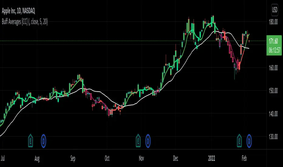
[blackcat] L1 Buff AverageLevel: 1
Background
This indicator buffs up your moving averages using the volume-weighting method presented in Buff Dormeier's article in 2001, "Buff Up Your Moving Averages." The weighting formula has been created as a function in pine script so that it can be referenced from any analysis technique or strategy. In addition, a simple two-line volume-weighted average indicator that references the function has also been included.
Function
The name of the volume-weighted average function is "BuffAverage()." The function has two inputs, price and length. The price input represents the price value upon which the average calculation is based. The length input represents the number of bars that are used in the calculation of the average. The two-line volume-weighted average indicator is presented. This indicator has three inputs. The price input represents the price value upon which the average calculation is based. The FastAvg input represents the number of bars to use in the fast volume-weighted average calculation. The SlowAvg input represents the number of bars to use in the slow volume-weighted average calculation. A simple alert criteria has also been included to provide an alert when the two lines cross.
Key Signal
FastBuff Line --> fast line in yellow;
SlowBuff Line --> slow line in fuchsia.
Remarks
This is a Level 1 free and open source indicator.
Feedbacks are appreciated.
