Multi Cycles Slope-Fit System MLMulti Cycles Predictive System : A Slope-Adaptive Ensemble
Executive Summary:
The MCPS-Slope (Multi Cycles Slope-Fit System) represents a paradigm shift from static technical analysis to adaptive, probabilistic market modeling. Unlike traditional indicators that rely on a single algorithm with fixed settings, this system deploys a "Mixture of Experts" (MoE) ensemble comprising 13 distinct cycle and trend algorithms.
Using a Gradient-Based Memory (GBM) learning engine, the system dynamically solves the "Cycle Mode" problem by real-time weighting. It aggressively curve-fits the Slope of component cycles to the Slope of the price action, rewarding algorithms that successfully predict direction while suppressing those that fail.
This is a non-repainting, adaptive oscillator designed to identify market regimes, pinpoint high-probability reversals via OB/OS logic, and visualize the aggregate consensus of advanced signal processing mathematics.
1. The Core Philosophy: Why "Slope" Matters:
In technical analysis, most traders focus on Levels (Price is above X) or Values (RSI is at 70). However, the primary driver of price action is Momentum, which is mathematically defined as the Rate of Change, or the Slope.
This script introduces a novel approach: Slope Fitting.
Instead of asking "Is the cycle high or low?", this system asks: "Is the trajectory (Slope) of this cycle matching the trajectory of the price?"
The Dual-Functionality of the Normalized Oscillator
The final output is a normalized oscillator bounded between -1.0 and +1.0. This structure serves two critical functions simultaneously:
Directional Bias (The Slope):
When the Combined Cycle line is rising (Positive Slope), the aggregate consensus of the 13 algorithms suggests bullish momentum. When falling (Negative Slope), it suggests bearish momentum. The script measures how well these slopes correlate with price action over a rolling lookback window to assign confidence weights.
Overbought / Oversold (OB/OS) Identification:
Because the output is mathematically clipped and normalized:
Approaching +1.0 (Overbought): Indicates that the top-weighted algorithms have reached their theoretical maximum amplitude. This is a statistical extreme, often preceding a mean reversion or trend exhaustion.
Approaching -1.0 (Oversold): Indicates the aggregate cycle has reached maximum bearish extension, signaling a potential accumulation zone.
Zero Line (0.0): The equilibrium point. A cross of the Zero Line is the most traditional signal of a trend shift.
2. The "Mixture of Experts" (MoE) Architecture:
Markets are dynamic. Sometimes they trend (Trend Following works), sometimes they chop (Mean Reversion works), and sometimes they cycle cleanly (Signal Processing works). No single indicator works in all regimes.
This system solves that problem by running 13 Algorithms simultaneously and voting on the outcome.
The 13 "Experts" Inside the Code:
All algorithms have been engineered to be Non-Repainting.
Ehlers Bandpass Filter: Extracts cycle components within a specific frequency bandwidth.
Schaff Trend Cycle: A double-smoothed stochastic of the MACD, excellent for cycle turning points.
Fisher Transform: Normalizes prices into a Gaussian distribution to pinpoint turning points.
Zero-Lag EMA (ZLEMA): Reduces lag to track price changes faster than standard MAs.
Coppock Curve: A momentum indicator originally designed for long-term market bottoms.
Detrended Price Oscillator (DPO): Removes trend to isolate short-term cycles.
MESA Adaptive (Sine Wave): Uses Phase accumulation to detect cycle turns.
Goertzel Algorithm: Uses Digital Signal Processing (DSP) to detect the magnitude of specific frequencies.
Hilbert Transform: Measures the instantaneous position of the cycle.
Autocorrelation: measures the correlation of the current price series with a lagged version of itself.
SSA (Simplified): Singular Spectrum Analysis approximation (Lag-compensated, non-repainting).
Wavelet (Simplified): Decomposes price into approximation and detail coefficients.
EMD (Simplified): Empirical Mode Decomposition approximation using envelope theory.
3. The Adaptive "GBM" Learning Engine
This is the "Machine Learning" component of the script. It does not use pre-trained weights; it learns live on your chart.
How it works:
Fitting Window: On every bar, the system looks back 20 days (configurable).
Slope Correlation: It calculates the correlation between the Slope of each of the 13 algorithms and the Slope of the Price.
Directional Bonus: It checks if the algorithm is pointing in the same direction as the price.
Weight Optimization:
Algorithms that match the price direction and correlation receive a higher "Fit Score."
Algorithms that diverge from price action are penalized.
A "Softmax" style temperature function and memory decay allow the weights to shift smoothly but aggressively.
The Result: If the market enters a clean sine-wave cycle, the Ehlers and Goertzel weights will spike. If the market explodes into a linear trend, ZLEMA and Schaff will take over, suppressing the cycle indicators that would otherwise call for a premature top.
4. How to Read the Interface:
The visual interface is designed for maximum information density without clutter.
The Dashboard (Bottom Left - GBM Stats)
Combined Fit: A percentage score (0-100%). High values (>70%) mean the system is "Locked In" and tracking price accurately. Low values suggest market chaos/noise.
Entropy: A measure of disorder. High entropy means the algorithms disagree (Neutral/Chop). Low entropy means the algorithms are unanimous (Strong Trend).
Top 1 / Top 3 Weight: Shows how concentrated the decision is. If Top 1 Weight is 50%, one algorithm is dominating the decision.
The Matrix (Bottom Right - Weight Table)
This table lifts the hood on the engine.
Fit Score: How well this specific algo is performing right now.
Corr/Dir: Raw correlation and Direction Match stats.
Weight: The actual percentage influence this algorithm has on the final line.
Cycle: The current value of that specific algorithm.
Regime: Identifies if the consensus is Bullish, Bearish, or Neutral.
The Chart Overlay
The Line: The Gradient-Colored line is the Weighted Ensemble Prediction.
Green: Bullish Slope.
Red: Bearish Slope.
Triangles: Zero-Cross signals (Bullish/Bearish).
"STRONG" Labels: Appears when the cycle sustains a value above +0.5 or below -0.5, indicating strong momentum.
Background Color: Changes subtly to reflect the aggregate Regime (Strong Up, Bullish, Neutral, Bearish, Strong Down).
5. Trading Strategies:
A. The Slope Reversal (OB/OS Fade)
Concept: Catching tops and bottoms using the -1/+1 normalization.
Signal: Wait for the Combined Cycle to reach extreme values (>0.8 or <-0.8).
Trigger: The entry is taken not when it hits the level, but when the Slope flips.
Short: Cycle hits +0.9, color turns from Green to Red (Slope becomes negative).
Long: Cycle hits -0.9, color turns from Red to Green (Slope becomes positive).
B. The Zero-Line Trend Join
Concept: Joining an established trend after a correction.
Signal: Price is trending, but the Cycle pulls back to the Zero line.
Trigger: A "Triangle" signal appears as the cycle crosses Zero in the direction of the higher timeframe trend.
C. Divergence Analysis
Concept: Using the "Fit Score" to identify weak moves.
Signal: Price makes a Higher High, but the Combined Cycle makes a Lower High.
Confirmation: Check the GBM Stats table. If "Combined Fit" is dropping while price is rising, the trend is decoupling from the cycle logic. This is a high-probability reversal warning.
6. Technical Configuration:
Fitting Window (Default: 20): The number of bars the ML engine looks back to judge algorithm performance. Lower (10-15) for scalping/quick adaptation. Higher (30-50) for swing trading and stability.
GBM Learning Rate (Default: 0.25): Controls how fast weights change.
High (>0.3): The system reacts instantly to new behaviors but may be "jumpy."
Low (<0.15): The system is very smooth but may lag in regime changes.
Max Single Weight (Default: 0.55): Prevents one single algorithm from completely hijacking the system, ensuring an ensemble effect remains.
Slope Lookback: The period over which the slope (velocity) is calculated.
7. Disclaimer & Notes:
Repainting: This indicator utilizes closed bar data for calculations and employs non-repainting approximations of SSA, EMD, and Wavelets. It does not repaint historical signals.
Calculations: The "ML" label refers to the adaptive weighting algorithm (Gradient-based optimization), not a neural network black box.
Risk: No indicator guarantees future performance. The "Fit Score" is a backward-looking metric of recent performance; market regimes can shift instantly. Always use proper risk management.
Author's Note
The MCPS-Slope was built to solve the frustration of "indicator shopping." Instead of switching between an RSI, a MACD, and a Stochastic depending on the day, this system mathematically determines which one is working best right now and presents you with a single, synthesized data stream.
If you find this tool useful, please leave a Boost and a Comment below!
Fishertransformspecial

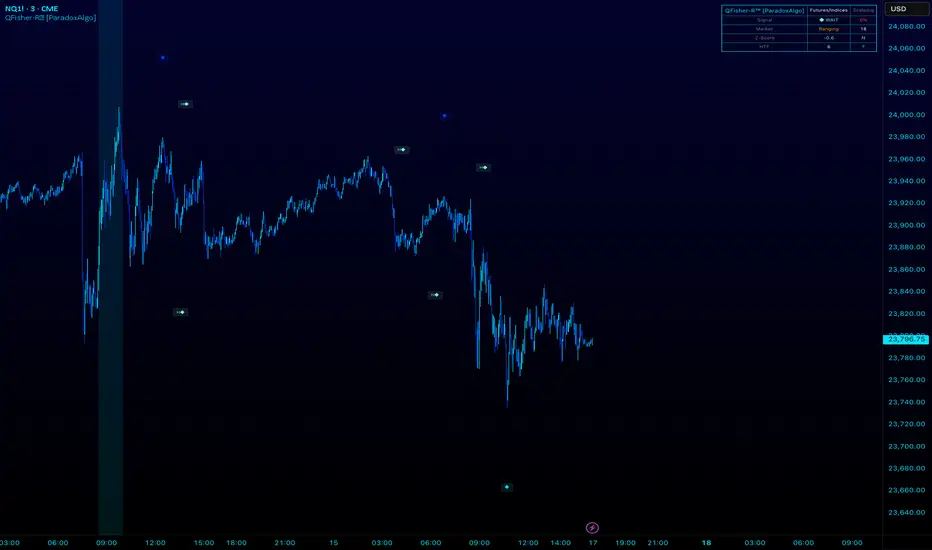
QFisher-R™ [ParadoxAlgo]QFISHER-R™ (Regime-Aware Fisher Transform)
A research/education tool that helps visualize potential momentum exhaustion and probable inflection zones using a quantitative, non-repainting Fisher framework with regime filters and multi-timeframe (MTF) confirmation.
What it does
Converts normalized price movement into a stabilized Fisher domain to highlight potential turning points.
Uses adaptive smoothing, robust (MAD/quantile) thresholds, and optional MTF alignment to contextualize extremes.
Provides a Reversal Probability Score (0–100) to summarize signal confluence (extreme, slope, cross, divergence, regime, and MTF checks).
Key features
Non-repainting logic (bar-close confirmation; security() with no lookahead).
Dynamic exhaustion bands (data-driven thresholds vs fixed ±2).
Adaptive smoothing (efficiency-ratio based).
Optional divergence tags on structurally valid pivots.
MTF confirmation (same logic computed on a higher timeframe).
Compact visuals with subtle plotting to reduce chart clutter.
Inputs (high level)
Source (e.g., HLC3 / Close / HA).
Core lookback, fast/slow range blend, and ER length.
Band sensitivity (robust thresholding).
MTF timeframe(s) and agreement requirement.
Toggle divergence & intrabar previews (default off).
Signals & Alerts
Turn Candidate (Up/Down) when multiple conditions align.
Trade-Grade Turn when score ≥ threshold and MTF agrees.
Divergence Confirmed when structural criteria are met.
Alerts are generated on confirmed bar close by default. Optional “preview” mode is available for experimentation.
How to use
Start on your preferred timeframe; optionally enable an HTF (e.g., 4×) for confirmation.
Look for RPS clusters near the exhaustion bands, slope inflections, and (optionally) divergences.
Combine with your own risk management, liquidity, and trend context.
Paper test first and calibrate thresholds to your instrument and timeframe.
Notes & limitations
This is not a buy/sell signal generator and does not predict future returns.
Readings can remain extreme during strong trends; use HTF context and your own filters.
Parameters are intentionally conservative by default; adjust carefully.
Compliance / Disclaimer
Educational & research tool only. Not financial advice. No recommendation to buy/sell any security or derivative.
Past performance, backtests, or examples (if any) are not indicative of future results.
Trading involves risk; you are responsible for your own decisions and risk management.
Built upon the Fisher Transform concept (Ehlers); all modifications, smoothing, regime logic, scoring, and visualization are original work by Paradox Algo.
SuperTrend Fisher [AlgoAlpha]🚀🌟 Introducing the "Super Fisher" by AlgoAlpha, a sophisticated and versatile tool crafted for the discerning trader. This innovative indicator merges the precision of the Fisher Transform with the adaptability of the SuperTrend methodology, offering a fresh perspective on market analysis. 📈🔍
Key Features:
🔶 Customizable Settings: Tailor the indicator to your trading style with adjustable inputs like "Fair-value Period" and "EMA Length". Choose your preferred "Up Color" and "Down Color" for a personalized visual experience.
🔶 Advanced Fisher Transform: At the heart of this tool is the Fisher Transform, an algorithm renowned for pinpointing potential price reversals by normalizing asset prices.
🔶 Integrated SuperTrend Functionality: This feature adds a layer of trend analysis, using the refined Fisher Transform values to generate dynamic, trend-following signals.
🔶 Enhanced Visualization: Clearly distinguishable bullish and bearish market phases, thanks to the color-coded plots of Fisher Transform and SuperTrend values.
🔶 Overbought/Oversold Levels: Visual plots and fills for these levels provide additional insights into market extremities.
🔶 Configurable Alerts: Stay informed with alerts for critical market movements like crossing the zero line or the SuperTrend.
Logic:
The "Super Fisher" operates on a sophisticated algorithm:
1. Fisher Transform Calculation: It starts by calculating the Detrended Price Oscillator (DPO) and its standard deviation. These values are then transformed using the Fisher Transform formula, which is subsequently smoothed with a Hull Moving Average.
2. SuperTrend Integration: The SuperTrend function employs the Fisher Transform values to create a dynamic trend-following tool. It calculates upper and lower bands and determines which one to use for market direction based on whether the fisher is above or below the bands, offering an insightful view of the price trend.
3. Overbought/Oversold Identification: The tool plots specific levels to indicate overbought and oversold conditions, aiding in the identification of potential reversal points.
Here's a closer look at the core calculations:
Calculates the Fisher Transform:
value = 0.0
value := round_(.66 * ((src - low_) / (high_ - low_) - .5) + .67 * nz(value ))
fish1 = 0.0
fish1 := .5 * math.log((1 + value) / (1 - value)) + .5 * nz(fish1 )
fish1 := ta.hma(fish1, l)
Calculates the SuperTrend:
supertrend(factor, atrPeriod, srcc) =>
src = srcc
atr = atrr(srcc, atrPeriod)
upperBand = src + factor * atr
lowerBand = src - factor * atr
prevLowerBand = nz(lowerBand )
prevUpperBand = nz(upperBand )
lowerBand := lowerBand > prevLowerBand or srcc < prevLowerBand ? lowerBand : prevLowerBand
upperBand := upperBand < prevUpperBand or srcc > prevUpperBand ? upperBand : prevUpperBand
int direction = na
float superTrend = na
prevSuperTrend = superTrend
if na(atr )
direction := 1
else if prevSuperTrend == prevUpperBand
direction := srcc > upperBand ? -1 : 1
else
direction := srcc < lowerBand ? 1 : -1
superTrend := direction == -1 ? lowerBand : upperBand
How to Use:
📊 To maximize the potential of the "Super Fisher", follow these steps:
1. Customize Settings: Adjust the inputs to match your trading preferences. This includes setting the periods for the Fisher Transform and SuperTrend, as well as choosing colors for better visualization.
2. Analyze the Market: Observe the Fisher Transform and SuperTrend plots to gauge market direction. Pay special attention to color changes, as they indicate shifts in market sentiment.
3. Identify Extremes: Use the overbought and oversold plots to understand potential reversal points.
4. Set Alerts: Utilize the alert functionality to stay informed about significant market movements, ensuring you never miss an opportunity.
🔥 In summary the "Super Fisher" is a comprehensive market analysis tool designed to enhance your trading insights and decision-making process. 📉🌟🚨
