Dynamic ATR-based Renko Overlay - Non repaintingDaily ATR-Based Renko Overlay
Overview
This Pine Script v5 indicator creates a dynamic Renko overlay on your time-based charts (optimized for 1-minute timeframes), using the previous period's ATR from a user-specified higher timeframe (default: 1-hour) to determine brick sizes. Unlike traditional Renko charts, this is an overlay that draws Renko bricks directly on top of your existing candles, allowing you to combine the noise-filtering power of Renko with the full features of time-based charts.
It's designed for traders who want Renko's trend-clarity benefits without switching chart types, especially useful for intraday trading in volatile markets like forex, stocks, or crypto.
Key Features
- Adaptive Brick Sizing: Brick size is calculated as a percentage (default 40%) of the previous period's ATR (Average True Range, default length 14) from the selected higher timeframe (default: 1-hour). This makes bricks volatility-adjusted—larger in high-vol periods to reduce noise, smaller in low-vol for more detail.
- Periodic Recalculation: Resets brick size at the start of each new period based on the user-specified reset timeframe (default: daily), using the prior period's ATR from the chosen timeframe. This ensures relevance without unwanted disruptions.
- Traditional Renko Logic: Uses 1-box reversal (a full brick against the trend to reverse). Bricks form based on closing prices, ignoring time and minor fluctuations.
- Visual Style: Stepped lines with green (up) and red (down) fills for a box-like appearance. Semi-transparent for easy overlay on candles.
- Customizable Inputs:
- ATR Length: Adjust the ATR period (default: 14).
- Percentage of ATR: Fine-tune brick sensitivity (default: 0.4 or 40%; range 0-1).
- ATR Timeframe: Specify the timeframe for ATR calculation (default: "60" for 1-hour; enter as a string like "240" for 4-hour, "D" for daily, etc.).
- Reset Timeframe: Specify the period for recalculating the brick size (default: "D" for daily; enter as a string like "W" for weekly, "M" for monthly, etc.).
How It Works
1. Fetches ATR from the user-specified timeframe via `request.security` for higher-timeframe volatility data.
2. On new periods based on the reset timeframe (or first load), sets brick size to `percent * ATR_HTF`.
3. Tracks Renko "close" and "previous close" to calculate bricks:
- Upward moves add green bricks in multiples of the size.
- Downward moves add red bricks.
- Reversals require a full brick against the direction.
4. Plots and fills create the overlay, updating on each 1-min bar close.
Add it to a 1-minute chart for best results—bricks will adapt periodically while you retain full candle visibility.
Why This Indicator is Helpful
TradingView's native Renko charts are powerful but come with limitations that can frustrate serious traders:
- No Bar Replay: Native Renko doesn't support TradingView's bar replay feature, making it hard to simulate historical trading sessions.
- Inaccurate/Repainting Strategy Testing: Strategies on native Renko can repaint or lack precision due to the non-time-based nature, leading to unreliable backtests.
- Limited Data History: Fast Renko timeframes (e.g., small bricks) often load very little historical data, restricting long-term analysis.
This overlay solves these by building Renko on a time-based chart:
- Full Bar Replay Support: Replay sessions as usual on your 1-min chart—the Renko follows along.
- Accurate, Non-Repainting Testing: Test strategies on the underlying time chart without repainting issues, as Renko is derived from closes.
- Unlimited Data Depth: Access TradingView's full historical data for 1-min charts (up to years of bars), not limited by Renko's data constraints.
- Hybrid Analysis: Overlay Renko on candles to spot trends while using volume, indicators (e.g., RSI, MAs), or drawing tools that don't work well on native Renko.
It's a game-changer for trend-following, breakout strategies, or filtering noise in short-term trades. No more switching charts—get the best of both worlds!
Usage Tips
- Best on 1-min charts for intraday precision, but experiment with others.
- Tune the percentage lower (e.g., 0.3) for more bricks/sensitivity, higher (e.g., 0.5) for fewer/false-signal reduction.
- Adjust the ATR timeframe to match your strategy—e.g., "240" for longer-term volatility or "15" for shorter.
- Customize the reset timeframe for different recalculation frequencies—e.g., "W" for weekly resets to capture broader market shifts, or "240" for every 4 hours.
- Combine with alerts: right now I am experimenting with 90 period EMA and the Renko brick pullbacks to find some EDGE
If you find this useful, give it a thumbs up or share your tweaks in the comments. Feedback welcome—happy trading! 🚀
Dynamic

Next Candle PredictorAdvanced TradingView Indicator for Precise Buy and Sell Signals
Overview:
The Predicta Futures - Next Candle Predictor is a cutting-edge TradingView indicator designed to forecast the next candle's direction in futures and cryptocurrency markets. Leveraging a multi-indicator confluence strategy, this tool provides traders with actionable long and short prediction percentages, enhanced by dynamic ADX-based thresholds and visual projection candles. Ideal for scalping, day trading, or swing trading on platforms like MEXC or Binance futures, it combines Supertrend, MACD, RSI, Stochastic, ADX, and volume analysis to deliver high-probability buy and sell signals while minimizing false positives.
Key Features:
* Multi-Indicator Confluence Scoring: Integrates Supertrend for trend direction, EMAs (8, 21, 50) for alignment, MACD for momentum crossovers, RSI for overbought/oversold conditions, Stochastic for divergence detection, ADX for trend strength, and volume ratios for confirmation. A customizable confluence score (0-6) ensures signals meet user-defined criteria, reducing whipsaws in volatile markets.
* Dynamic Prediction Thresholds: ADX-driven adjustments lower the required prediction percentage (e.g., 60% in strong trends) for "PERFECT TIME" entries, adapting to market conditions like ranging or trending phases.
* Visual Analysis Table: A sleek, color-coded dashboard displays progress bars for each indicator, prediction percentages, and status (e.g., "PERFECT TIME" or "WAIT"). Supports long and short analyses with intuitive ASCII bars for quick scans.
* Projection Candles: Simulates potential next-candle outcomes with volatility-scaled (via Bollinger Bands width) green long and red short candles, aiding in visualizing price targets.
Buy/Sell Signals and Alerts: Generates labeled "BUY" and "SELL" arrows on EMA crossovers within confirmed trends, with separate alerts for basic signals and high-confluence "PERFECT TIME" opportunities.
* Customizable Inputs: Adjust ATR periods, Supertrend factors, minimum confluence scores, and volume ratios to tailor the indicator for stocks, forex, or crypto perpetual futures.
How It Works:
This TradingView script calculates long and short scores using weighted contributions from key indicators, normalizing them into prediction percentages. A confluence check—factoring trend, EMA alignment, MACD, Stochastic, volume, and ADX—triggers "PERFECT TIME" only when conditions align robustly. For example:
In a downtrend (Supertrend red), with bearish MACD and Stochastic, and sufficient volume, the indicator highlights short opportunities.
Dynamic thresholds ensure aggressive entries in strong trends (ADX >25) and conservative ones in weak trends.
Backtested for reliability, it excels in identifying reversals and continuations, making it a must-have for traders seeking an edge in futures trading strategies.
Usage Instructions:
1. Add the indicator to your TradingView chart.
2. Customize settings via the inputs panel (e.g., set minConfluence to 5 for stricter signals).
3. Monitor the analysis table for predictions and confluence scores.
4. Act on "BUY/SELL" labels or "PERFECT TIME" alerts, combining with your risk management.
5. Enable projection candles for visual forecasting of the next bar.
Compatible with all timeframes, from 1-minute scalping to daily swings. Note: This is not financial advice; always verify signals with additional analysis.
Rate and review if it boosts your trades!
Thank you!

TDI Fibonacci Volatility Bands Candle Coloring [cryptalent]"This is an advanced Traders Dynamic Index (TDI) candle coloring system, designed for traders seeking precise dynamic analysis. Unlike traditional TDI, which typically relies on a 50 midline with a single standard deviation band (±1 SD), this indicator innovatively incorporates Fibonacci golden ratio multiples (1.618, 2.618, 3.618 times standard deviation) to create multi-layered dynamic bands. It precisely divides the RSI fast line (green line) position into five distinct strength zones, instantly reflecting them on the candle colors, allowing you to grasp market sentiment in real-time without switching to a sub-chart.
Core Calculation Logic:
RSI Period (default 20), Band Length (default 50), and Fast MA Smoothing Period (default 1) are all adjustable.
The midline is the Simple Moving Average (SMA) of RSI, with upper and lower bands calculated by multiplying Fibonacci multiples with Standard Deviation (STDEV), generating three dynamic band sets: 1.618, 2.618, and 3.618.
Traders can quickly identify the following scenarios:
Extreme Overbought Zone (Strong Bullish, Red): Fast line exceeds custom threshold (default 82) and breaks above the specified band (default 2.618). This often signals overheating, potentially a profit-taking point or reversal short entry, especially at trend tops.
Extreme Oversold Zone (Strong Bearish, Green): Fast line drops below custom threshold (default 28) and breaks below the specified band (default 2.618). This is a potential strong rebound starting point, ideal for bottom-fishing or long entries.
Medium Bullish Zone (Yellow): Fast line surpasses medium threshold (default 66) and stands above the specified band (default 1.618), indicating bullish dominance in trend continuation.
Medium Bearish Zone (Orange): Fast line falls below medium threshold (default 33) and breaks below the specified band (default 1.618), signaling bearish control in segment transitions.
Neutral Zone (No Color Change): Fast line within custom upper and lower limits (default 34~65), retaining original candle colors to avoid noise interference during consolidation.
Color priority logic flows from strong to weak (Extreme > Medium > Neutral), ensuring no conflicts. All parameters are highly customizable, including thresholds, band selections (1.618/2.618/3.618/Midline/None), color schemes, and even optional semi-transparent background coloring (default off, transparency 90%) for enhanced visual layering.
Applicable Scenarios:
Intraday Trading: Capture extreme color shifts as entry/exit signals.
Swing Trading: Use medium colors to confirm trend extensions.
Long-Term Trend Following: Filter noise in neutral zones to focus on major trends.
Supports various markets like forex, stocks, and cryptocurrencies. After installation, adjust parameters in settings to match your strategy, and combine with other indicators like moving averages or support/resistance for improved accuracy.
If you're a TDI enthusiast, this will make your trading more intuitive and efficient!

Dynamic 15-Ticker Multi-Symbol Table 2025 EditionTitle:
Dynamic 15-Ticker Multi-Symbol Table 2025 Edition
Description:
This script provides a multi-ticker table for TradingView charts. It is fully open-source and free to use. The table displays up to 15 tickers, including SPY as the baseline symbol. The script updates in real-time on any timeframe.
Features:
SPY baseline: The first row always shows SPY for reference.
Custom tickers: Add up to 14 additional tickers via the input settings. Rows without tickers remain hidden.
Price and direction: Each ticker row displays the current price and an indicator of direction based on recent price movement.
RSI (14) indicator: Shows the current relative strength index value with a simple directional marker.
Volume formatting: Displays volume values in thousands, millions, or billions automatically. Volume change is indicated with directional markers.
Stable layout: The table uses alternating row colors for readability and maintains consistent row count without collapsing or disappearing rows.
Real-time updates: All displayed values refresh automatically on any chart timeframe.
How to use:
Add the script to your chart.
Enter your chosen tickers in the input settings. SPY will remain as the first ticker automatically.
Tickers not entered will remain hidden. When a ticker is removed, the row will be removed-dynamically.
Observe live prices, RSI values, and volume changes directly on your chart without switching symbols.
Additional notes:
The script is fully open-source; users are encouraged to modify or improve it.
No external links or references are required to understand its function.
This script does not repaint and does not require additional requests to update values.

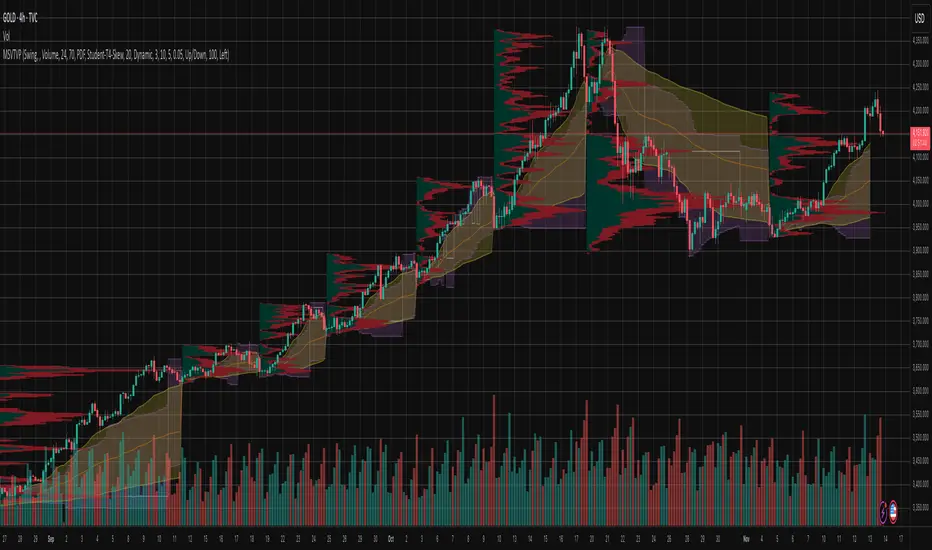
Market Structure Volume Time Velocity ProfileThis is the Market Structure Volume Time Velocity Profile (MSVTVP). It combines event-based profiling with advanced metrics like Time and Velocity (Flow Rate). Instead of fixed time periods, profiles are anchored to critical market events (Swings, Structure Breaks, Delta Breaks), giving you a precise view of value development during specific market phases.
## The 3 Dimensions of the Market
Unlike standard tools that only show Volume, MSVTVP allows you
to switch between three critical metrics:
1. **VOLUME Profile (The "Where"):**
* Shows standard acceptance. High volume nodes (HVN)
are magnets for price.
2. **TIME Profile (The "How Long"):**
* Similar to TPO, it measures how long price spent at each
level.
* **High Time:** True acceptance and fair value.
* **Low Time:** Rejection or rapid movement.
3. **VELOCITY Profile (The "How Fast"):**
* Measures the **speed of trading** (Contracts per Second).
This reveals the hidden intent of market participants.
* **High Velocity (Fast Flow):** Aggression. Initiative
buyers/sellers are hitting market orders rapidly. Often
seen at breakouts or in liquidity vacu.
* **Low Velocity (Slow Flow):** Absorption. Massive passive
limit orders are slowing price down despite high volume.
Often seen at major reversals ("hitting a brick wall").
Key Features:
1. **Event-Based Profile Anchoring:** The indicator starts a new
profile based on one of three user-selected events
('Profile Anchor'):
- **Swing:** A new profile begins when the 'impulse baseline'
(derived from intra-bar delta) changes. This baseline
adjusts when a new **price pivot** is confirmed: When a
price **high** forms, the baseline moves to the **lower**
of its previous level or the peak delta (max of
delta O/C) at the pivot. When a price **low** forms, it
moves to the **higher** of its previous level or the
trough delta (min of delta O/C) at the pivot.
- **Structure:** A new profile begins immediately on the bar
that *confirms* a market structure break (e.g., a new HH
or LL, based on a sequence of price pivots).
- **Delta:** A new profile begins immediately on the bar
that *confirms* a break in the *cumulative delta's*
market structure (e.g., a new HH or LL in the delta).
Both 'Swing' and 'Delta' anchors are derived from the same
**continuous (non-resetting) Cumulative Volume Profile Delta (CVPD)**,
which is built from the intra-bar statistical analysis.
2. **Statistical Profile Engine:** For each bar in the anchored
period, the indicator builds a volume profile on a lower
'Intra-Bar Timeframe'. Instead of simple tick counting, it
uses advanced statistical models:
- **Allocation ('Allot model'):** 'PDF' (Probability Density
Function) distributes volume proportionally across the
bar's range based on an assumed statistical model
(e.g., T4-Skew). 'Classic' assigns all volume to
the close.
- **Buy/Sell Split ('Volume Estimator'):** 'Dynamic'
applies a model that analyzes candle wicks and
recent trend to estimate buy/sell pressure. 'Classic'
classifies all volume based on the candle color.
3. **Visualization & Lag:** The indicator plots the final
profile (as a polygon) and the developing statistical
lines (POC, VA, VWAP, StdDev).
- **Note on Lag:** All anchor events require `Pivot Right Bars`
for confirmation.
- In 'Structure' and 'Delta' mode, the developing lines
(POC, VA, etc.) are plotted using a **non-repainting**
method (showing the value from `pivRi` bars ago).
- In 'Swing' mode, the profile is plotted **retroactively**,
starting *from the bar where the pivot occurred*. The
developing lines are also plotted with this full
`pivRi` lag to align with the past data.
4. **Flexible Display Modes:** The finalized profile can be displayed
in three ways: 'Up/Down' (buy vs. sell), 'Total' (combined
volume), and 'Delta' (net difference).
5. **Dynamic Row Sizing:** Includes an option ('Rows per Percent')
to automatically adjust the number of profile rows (buckets)
based on the profile's price range.
6. **Integrated Alerts:** Includes 13 alerts that trigger for:
- A new profile reset ('Profile was resetted').
- Price crossing any of the 6 developing levels (POC,
VA High/Low, VWAP, StdDev High/Low).
- **Alert Lag Assumption:** In 'Swing' mode, alerts are
delayed to match the retroactively plotted lines.
In 'Structure' and 'Delta' modes, alerts fire in
**real-time** based on the *current price* crossing
the *current (repainting)* value of the metric, which
may **differ from the non-repainting plotted line.**
**Caution: Real-Time Data Behavior (Intra-Bar Repainting)**
This indicator uses high-resolution intra-bar data. As a result, the
values on the **current, unclosed bar** (the real-time bar) will
update dynamically as new intra-bar data arrives. This includes
the values used for real-time alerts in 'Structure' and
'Delta' modes.
---
**DISCLAIMER**
1. **For Informational/Educational Use Only:** This indicator is
provided for informational and educational purposes only. It does
not constitute financial, investment, or trading advice, nor is
it a recommendation to buy or sell any asset.
2. **Use at Your Own Risk:** All trading decisions you make based on
the information or signals generated by this indicator are made
solely at your own risk.
3. **No Guarantee of Performance:** Past performance is not an
indicator of future results. The author makes no guarantee
regarding the accuracy of the signals or future profitability.
4. **No Liability:** The author shall not be held liable for any
financial losses or damages incurred directly or indirectly from
the use of this indicator.
5. **Signals Are Not Recommendations:** The alerts and visual signals
(e.g., crossovers) generated by this tool are not direct
recommendations to buy or sell. They are technical observations
for your own analysis and consideration.
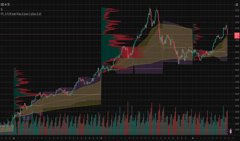
Periodic Volume Time Velocity ProfileThis is the Periodic Volume Time Velocity Profile (PVTVP). It is an advanced professional profiling tool that goes beyond standard volume analysis by introducing Time and Velocity (Flow Rate) as profile dimensions.
By analyzing high-resolution intra-bar data, it builds
precise profiles for any custom period (Session, Day, Week, etc.),
helping you understand not just *where* the market traded,
but *how* it traded there.
## The 3 Dimensions of the Market
Unlike standard tools that only show Volume, PVTVP allows you
to switch between three critical metrics:
1. **VOLUME Profile (The "Where"):**
* Shows standard acceptance. High volume nodes (HVN)
are magnets for price.
2. **TIME Profile (The "How Long"):**
* Similar to TPO, it measures how long price spent at each
level.
* **High Time:** True acceptance and fair value.
* **Low Time:** Rejection or rapid movement.
3. **VELOCITY Profile (The "How Fast"):**
* Measures the **speed of trading** (Contracts per Second).
This reveals the hidden intent of market participants.
* **High Velocity (Fast Flow):** Aggression. Initiative
buyers/sellers are hitting market orders rapidly. Often
seen at breakouts or in liquidity vacuums.
* **Low Velocity (Slow Flow):** Absorption. Massive passive
limit orders are slowing price down despite high volume.
Often seen at major reversals ("hitting a brick wall").
## Key Features
1. **Statistical Volume Profile Engine:** For each bar in the selected
period, the indicator builds a complete volume profile on a lower
'Intra-Bar Timeframe'. Instead of simple tick counting, it uses
**statistical models ('PDF' allocation)** to distribute volume
across price levels and **advanced classifiers ('Dynamic' split)**
to determine the buy/sell pressure within that profile.
2. **Flexible Profile Display:** The **finalized profile** (plotted at
the end of each period) can be visualized in three distinct
ways: 'Up/Down' (buy vs. sell), 'Total' (combined volume),
and 'Delta' (net difference).
3. **Developing Key Levels:** The indicator also plots the developing
Point of Control (POC), Value Area (VA), VWAP, and Standard
Deviation bands in real-time as the period unfolds, providing
live insights into the emerging market structure.
4. **Dynamic Row Sizing:** Includes an option ('Rows per Percent')
to automatically adjust the number of profile rows (buckets)
based on the profile's price range, maintaining a consistent
visual density.
5. **Integrated Alerts:** Includes 12 alerts that trigger when the
main price crosses over or under the key developing levels:
POC, VWAP, Value Area High/Low, and the +/- Standard
Deviation bands.
**Caution: Real-Time Data Behavior (Intra-Bar Repainting)**
This indicator uses high-resolution intra-bar data. As a result, the
values on the **current, unclosed bar** (the real-time bar) will
update dynamically as new intra-bar data arrives. This behavior is
normal and necessary for this type of analysis. Signals should only
be considered final **after the main chart bar has closed.**
---
**DISCLAIMER**
1. **For Informational/Educational Use Only:** This indicator is
provided for informational and educational purposes only. It does
not constitute financial, investment, or trading advice, nor is
it a recommendation to buy or sell any asset.
2. **Use at Your Own Risk:** All trading decisions you make based on
the information or signals generated by this indicator are made
solely at your own risk.
3. **No Guarantee of Performance:** Past performance is not an
indicator of future results. The author makes no guarantee
regarding the accuracy of the signals or future profitability.
4. **No Liability:** The author shall not be held liable for any
financial losses or damages incurred directly or indirectly from
the use of this indicator.
5. **Signals Are Not Recommendations:** The alerts and visual signals
(e.g., crossovers) generated by this tool are not direct
recommendations to buy or sell. They are technical observations
for your own analysis and consideration.

Volatility-Targeted Momentum Portfolio [BackQuant]Volatility-Targeted Momentum Portfolio
A complete momentum portfolio engine that ranks assets, targets a user-defined volatility, builds long, short, or delta-neutral books, and reports performance with metrics, attribution, Monte Carlo scenarios, allocation pie, and efficiency scatter plots. This description explains the theory and the mechanics so you can configure, validate, and deploy it with intent.
Table of contents
What the script does at a glance
Momentum, what it is, how to know if it is present
Volatility targeting, why and how it is done here
Portfolio construction modes: Long Only, Short Only, Delta Neutral
Regime filter and when the strategy goes to cash
Transaction cost modelling in this script
Backtest metrics and definitions
Performance attribution chart
Monte Carlo simulation
Scatter plot analysis modes
Asset allocation pie chart
Inputs, presets, and deployment checklist
Suggested workflow
1) What the script does at a glance
Pulls a list of up to 15 tickers, computes a simple momentum score on each over a configurable lookback, then volatility-scales their bar-to-bar return stream to a target annualized volatility.
Ranks assets by raw momentum, selects the top 3 and bottom 3, builds positions according to the chosen mode, and gates exposure with a fast regime filter.
Accumulates a portfolio equity curve with risk and performance metrics, optional benchmark buy-and-hold for comparison, and a full alert suite.
Adds visual diagnostics: performance attribution bars, Monte Carlo forward paths, an allocation pie, and scatter plots for risk-return and factor views.
2) Momentum: definition, detection, and validation
Momentum is the tendency of assets that have performed well to continue to perform well, and of underperformers to continue underperforming, over a specific horizon. You operationalize it by selecting a horizon, defining a signal, ranking assets, and trading the leaders versus laggards subject to risk constraints.
Signal choices . Common signals include cumulative return over a lookback window, regression slope on log-price, or normalized rate-of-change. This script uses cumulative return over lookback bars for ranking (variable cr = price/price - 1). It keeps the ranking simple and lets volatility targeting handle risk normalization.
How to know momentum is present .
Leaders and laggards persist across adjacent windows rather than flipping every bar.
Spread between average momentum of leaders and laggards is materially positive in sample.
Cross-sectional dispersion is non-trivial. If everything is flat or highly correlated with no separation, momentum selection will be weak.
Your validation should include a diagnostic that measures whether returns are explained by a momentum regression on the timeseries.
Recommended diagnostic tool . Before running any momentum portfolio, verify that a timeseries exhibits stable directional drift. Use this indicator as a pre-check: It fits a regression to price, exposes slope and goodness-of-fit style context, and helps confirm if there is usable momentum before you force a ranking into a flat regime.
3) Volatility targeting: purpose and implementation here
Purpose . Volatility targeting seeks a more stable risk footprint. High-vol assets get sized down, low-vol assets get sized up, so each contributes more evenly to total risk.
Computation in this script (per asset, rolling):
Return series ret = log(price/price ).
Annualized volatility estimate vol = stdev(ret, lookback) * sqrt(tradingdays).
Leverage multiplier volMult = clamp(targetVol / vol, 0.1, 5.0).
This caps sizing so extremely low-vol assets don’t explode weight and extremely high-vol assets don’t go to zero.
Scaled return stream sr = ret * volMult. This is the per-bar, risk-adjusted building block used in the portfolio combinations.
Interpretation . You are not levering your account on the exchange, you are rescaling the contribution each asset’s daily move has on the modeled equity. In live trading you would reflect this with position sizing or notional exposure.
4) Portfolio construction modes
Cross-sectional ranking . Assets are sorted by cr over the chosen lookback. Top and bottom indices are extracted without ties.
Long Only . Averages the volatility-scaled returns of the top 3 assets: avgRet = mean(sr_top1, sr_top2, sr_top3). Position table shows per-asset leverages and weights proportional to their current volMult.
Short Only . Averages the negative of the volatility-scaled returns of the bottom 3: avgRet = mean(-sr_bot1, -sr_bot2, -sr_bot3). Position table shows short legs.
Delta Neutral . Long the top 3 and short the bottom 3 in equal book sizes. Each side is sized to 50 percent notional internally, with weights within each side proportional to volMult. The return stream mixes the two sides: avgRet = mean(sr_top1,sr_top2,sr_top3, -sr_bot1,-sr_bot2,-sr_bot3).
Notes .
The selection metric is raw momentum, the execution stream is volatility-scaled returns. This separation is deliberate. It avoids letting volatility dominate ranking while still enforcing risk parity at the return contribution stage.
If everything rallies together and dispersion collapses, Long Only may behave like a single beta. Delta Neutral is designed to extract cross-sectional momentum with low net beta.
5) Regime filter
A fast EMA(12) vs EMA(21) filter gates exposure.
Long Only active when EMA12 > EMA21. Otherwise the book is set to cash.
Short Only active when EMA12 < EMA21. Otherwise cash.
Delta Neutral is always active.
This prevents taking long momentum entries during obvious local downtrends and vice versa for shorts. When the filter is false, equity is held flat for that bar.
6) Transaction cost modelling
There are two cost touchpoints in the script.
Per-bar drag . When the regime filter is active, the per-bar return is reduced by fee_rate * avgRet inside netRet = avgRet - (fee_rate * avgRet). This models proportional friction relative to traded impact on that bar.
Turnover-linked fee . The script tracks changes in membership of the top and bottom baskets (top1..top3, bot1..bot3). The intent is to charge fees when composition changes. The template counts changes and scales a fee by change count divided by 6 for the six slots.
Use case: increase fee_rate to reflect taker fees and slippage if you rebalance every bar or trade illiquid assets. Reduce it if you rebalance less often or use maker orders.
Practical advice .
If you rebalance daily, start with 5–20 bps round-trip per switch on liquid futures and adjust per venue.
For crypto perp microcaps, stress higher cost assumptions and add slippage buffers.
If you only rotate on lookback boundaries or at signals, use alert-driven rebalances and lower per-bar drag.
7) Backtest metrics and definitions
The script computes a standard set of portfolio statistics once the start date is reached.
Net Profit percent over the full test.
Max Drawdown percent, tracked from running peaks.
Annualized Mean and Stdev using the chosen trading day count.
Variance is the square of annualized stdev.
Sharpe uses daily mean adjusted by risk-free rate and annualized.
Sortino uses downside stdev only.
Omega ratio of sum of gains to sum of losses.
Gain-to-Pain total gains divided by total losses absolute.
CAGR compounded annual growth from start date to now.
Alpha, Beta versus a user-selected benchmark. Beta from covariance of daily returns, Alpha from CAPM.
Skewness of daily returns.
VaR 95 linear-interpolated 5th percentile of daily returns.
CVaR average of the worst 5 percent of daily returns.
Benchmark Buy-and-Hold equity path for comparison.
8) Performance attribution
Cumulative contribution per asset, adjusted for whether it was held long or short and for its volatility multiplier, aggregated across the backtest. You can filter to winners only or show both sides. The panel is sorted by contribution and includes percent labels.
9) Monte Carlo simulation
The panel draws forward equity paths from either a Normal model parameterized by recent mean and stdev, or non-parametric bootstrap of recent daily returns. You control the sample length, number of simulations, forecast horizon, visibility of individual paths, confidence bands, and a reproducible seed.
Normal uses Box-Muller with your seed. Good for quick, smooth envelopes.
Bootstrap resamples realized returns, preserving fat tails and volatility clustering better than a Gaussian assumption.
Bands show 10th, 25th, 75th, 90th percentiles and the path mean.
10) Scatter plot analysis
Four point-cloud modes, each plotting all assets and a star for the current portfolio position, with quadrant guides and labels.
Risk-Return Efficiency . X is risk proxy from leverage, Y is expected return from annualized momentum. The star shows the current book’s composite.
Momentum vs Volatility . Visualizes whether leaders are also high vol, a cue for turnover and cost expectations.
Beta vs Alpha . X is a beta proxy, Y is risk-adjusted excess return proxy. Useful to see if leaders are just beta.
Leverage vs Momentum . X is volMult, Y is momentum. Shows how volatility targeting is redistributing risk.
11) Asset allocation pie chart
Builds a wheel of current allocations.
Long Only, weights are proportional to each long asset’s current volMult and sum to 100 percent.
Short Only, weights show the short book as positive slices that sum to 100 percent.
Delta Neutral, 50 percent long and 50 percent short books, each side leverage-proportional.
Labels can show asset, percent, and current leverage.
12) Inputs and quick presets
Core
Portfolio Strategy . Long Only, Short Only, Delta Neutral.
Initial Capital . For equity scaling in the panel.
Trading Days/Year . 252 for stocks, 365 for crypto.
Target Volatility . Annualized, drives volMult.
Transaction Fees . Per-bar drag and composition change penalty, see the modelling notes above.
Momentum Lookback . Ranking horizon. Shorter is more reactive, longer is steadier.
Start Date . Ensure every symbol has data back to this date to avoid bias.
Benchmark . Used for alpha, beta, and B&H line.
Diagnostics
Metrics, Equity, B&H, Curve labels, Daily return line, Rolling drawdown fill.
Attribution panel. Toggle winners only to focus on what matters.
Monte Carlo mode with Normal or Bootstrap and confidence bands.
Scatter plot type and styling, labels, and portfolio star.
Pie chart and labels for current allocation.
Presets
Crypto Daily, Long Only . Lookback 25, Target Vol 50 percent, Fees 10 bps, Regime filter on, Metrics and Drawdown on. Monte Carlo Bootstrap with Recent 200 bars for bands.
Crypto Daily, Delta Neutral . Lookback 25, Target Vol 50 percent, Fees 15–25 bps, Regime filter always active for this mode. Use Scatter Risk-Return to monitor efficiency and keep the star near upper left quadrants without drifting rightward.
Equities Daily, Long Only . Lookback 60–120, Target Vol 15–20 percent, Fees 5–10 bps, Regime filter on. Use Benchmark SPX and watch Alpha and Beta to keep the book from becoming index beta.
13) Suggested workflow
Universe sanity check . Pick liquid tickers with stable data. Thin assets distort vol estimates and fees.
Check momentum existence . Run on your timeframe. If slope and fit are weak, widen lookback or avoid that asset or timeframe.
Set risk budget . Choose a target volatility that matches your drawdown tolerance. Higher target increases turnover and cost sensitivity.
Pick mode . Long Only for bull regimes, Short Only for sustained downtrends, Delta Neutral for cross-sectional harvesting when index direction is unclear.
Tune lookback . If leaders rotate too often, lengthen it. If entries lag, shorten it.
Validate cost assumptions . Increase fee_rate and stress Monte Carlo. If the edge vanishes with modest friction, refine selection or lengthen rebalance cadence.
Run attribution . Confirm the strategy’s winners align with intuition and not one unstable outlier.
Use alerts . Enable position change, drawdown, volatility breach, regime, momentum shift, and crash alerts to supervise live runs.
Important implementation details mapped to code
Momentum measure . cr = price / price - 1 per symbol for ranking. Simplicity helps avoid overfitting.
Volatility targeting . vol = stdev(log returns, lookback) * sqrt(tradingdays), volMult = clamp(targetVol / vol, 0.1, 5), sr = ret * volMult.
Selection . Extract indices for top1..top3 and bot1..bot3. The arrays rets, scRets, lev_vals, and ticks_arr track momentum, scaled returns, leverage multipliers, and display tickers respectively.
Regime filter . EMA12 vs EMA21 switch determines if the strategy takes risk for Long or Short modes. Delta Neutral ignores the gate.
Equity update . Equity multiplies by 1 + netRet only when the regime was active in the prior bar. Buy-and-hold benchmark is computed separately for comparison.
Tables . Position tables show current top or bottom assets with leverage and weights. Metric table prints all risk and performance figures.
Visualization panels . Attribution, Monte Carlo, scatter, and pie use the last bars to draw overlays that update as the backtest proceeds.
Final notes
Momentum is a portfolio effect. The edge comes from cross-sectional dispersion, adequate risk normalization, and disciplined turnover control, not from a single best asset call.
Volatility targeting stabilizes path but does not fix selection. Use the momentum regression link above to confirm structure exists before you size into it.
Always test higher lag costs and slippage, then recheck metrics, attribution, and Monte Carlo envelopes. If the edge persists under stress, you have something robust.

Intra Bar Volume ProfileThis indicator provides a high-resolution volume profile analysis for every single bar on the chart. It builds this profile by sampling data from a lower intra-bar timeframe, allowing for a granular view of price distribution and buying/selling pressure within the bar.
Key Features:
Intra-Bar Profile Engine: For each bar on the main chart, the indicator builds a complete volume profile on a lower 'Intra-Bar Timeframe'. It uses:
Statistical Models ('Allot model'): Distributes volume across price levels using 'PDF' (Probability Density Function) or 'Classic' (close) methods.
Buy/Sell Classifiers ('Volume Estimator'): Splits volume using a 'Dynamic' (trend/wick-based) or 'Classic' (candle color) model.
On-Chart Visualization (Overlay): The analysis is rendered directly onto the price bars:
Point of Control (POC): A line showing the price level with the most volume for that bar.
Value Area (VA): A colored box representing the price range where the specified percentage (e..g., 50%) of volume was traded.
VWAP: Displays the volume-weighted average price (VWAP) for the bar as a separate line.
Integrated Alerts: Includes 8 alerts that trigger when the main price crosses over or under the key intra-bar levels: POC, VWAP, and the Value Area High/Low.
Caution: Real-Time Data Behavior (Intra-Bar Repainting) This indicator uses high-resolution intra-bar data. As a result, the values on the current, unclosed bar (the real-time bar) will update dynamically as new intra-bar data arrives. This behavior is normal and necessary for this type of analysis. Signals should only be considered final after the main chart bar has closed.
DISCLAIMM
For Informational/Educational Use Only: This indicator is provided for informational and educational purposes only. It does not constitute financial, investment, or trading advice, nor is it a recommendation to buy or sell any asset.
Use at Your Own Risk: All trading decisions you make based on the information or signals generated by this indicator are made solely at your own risk.
No Guarantee of Performance: Past performance is not an indicator of future results. The author makes no guarantee regarding the accuracy of the signals or future profitability.
No Liability: The author shall not be held liable for any financial losses or damages incurred directly or indirectly from the use of this indicator.
Signals Are Not Recommendations: The alerts and visual signals (e.g., crossovers) generated by this tool are not direct recommendations to buy or sell. They are technical observations for your own analysis and consideration.

Market Structure Volume ProfileThis indicator visualizes volume profiles that are dynamically anchored to market structure events, rather than fixed time intervals. It builds these profiles using high-resolution intra-bar data to provide a precise view of where value is established during critical market phases.
Key Features:
Event-Based Profile Anchoring: The indicator starts a new profile based on one of three user-selected events ('Profile Anchor'):
Swing: A new profile begins when the 'impulse baseline' (derived from intra-bar delta) changes. This baseline adjusts when a new price pivot is confirmed: When a price high forms, the baseline moves to the lower of its previous level or the peak delta (max of delta O/C) at the pivot. When a price low forms, it moves to the higher of its previous level or the trough delta (min of delta O/C) at the pivot.
Structure: A new profile begins immediately on the bar that confirms a market structure break (e.g., a new HH or LL, based on a sequence of price pivots).
Delta: A new profile begins immediately on the bar that confirms a break in the cumulative delta's market structure (e.g., a new HH or LL in the delta). Both 'Swing' and 'Delta' anchors are derived from the same continuous (non-resetting) Cumulative Volume Profile Delta (CVPD), which is built from the intra-bar statistical analysis.
Statistical Profile Engine: For each bar in the anchored period, the indicator builds a volume profile on a lower 'Intra-Bar Timeframe'. Instead of simple tick counting, it uses advanced statistical models:
Allocation ('Allot model'): 'PDF' (Probability Density Function) distributes volume proportionally across the bar's range based on an assumed statistical model (e.g., T4-Skew). 'Classic' assigns all volume to the close.
Buy/Sell Split ('Volume Estimator'): 'Dynamic' applies a model that analyzes candle wicks and recent trend to estimate buy/sell pressure. 'Classic' classifies all volume based on the candle color.
Visualization & Lag: The indicator plots the final profile (as a polygon) and the developing statistical lines (POC, VA, VWAP, StdDev).
Note on Lag: All anchor events require Pivot Right Bars for confirmation.
In 'Structure' and 'Delta' mode, the developing lines (POC, VA, etc.) are plotted using a non-repainting method (showing the value from pivRi bars ago).
In 'Swing' mode, the profile is plotted retroactively, starting from the bar where the pivot occurred. The developing lines are also plotted with this full pivRi lag to align with the past data.
Flexible Display Modes: The finalized profile can be displayed in three ways: 'Up/Down' (buy vs. sell), 'Total' (combined volume), and 'Delta' (net difference).
Dynamic Row Sizing: Includes an option ('Rows per Percent') to automatically adjust the number of profile rows (buckets) based on the profile's price range.
Integrated Alerts: Includes 13 alerts that trigger for:
A new profile reset ('Profile was resetted').
Price crossing any of the 6 developing levels (POC, VA High/Low, VWAP, StdDev High/Low).
Alert Lag Assumption: In 'Swing' mode, alerts are delayed to match the retroactively plotted lines. In 'Structure' and 'Delta' modes, alerts fire in real-time based on the current price crossing the current (repainting) value of the metric, which may differ from the non-repainting plotted line.
Caution: Real-Time Data Behavior (Intra-Bar Repainting) This indicator uses high-resolution intra-bar data. As a result, the values on the current, unclosed bar (the real-time bar) will update dynamically as new intra-bar data arrives. This includes the values used for real-time alerts in 'Structure' and 'Delta' modes.
DISCLAIMER
For Informational/Educational Use Only: This indicator is provided for informational and educational purposes only. It does not constitute financial, investment, or trading advice, nor is it a recommendation to buy or sell any asset.
Use at Your Own Risk: All trading decisions you make based on the information or signals generated by this indicator are made solely at your own risk.
No Guarantee of Performance: Past performance is not an indicator of future results. The author makes no guarantee regarding the accuracy of the signals or future profitability.
No Liability: The author shall not be held liable for any financial losses or damages incurred directly or indirectly from the use of this indicator.
Signals Are Not Recommendations: The alerts and visual signals (e.g., crossovers) generated by this tool are not direct recommendations to buy or sell. They are technical observations for your own analysis and consideration.

Periodic Volume ProfileThis indicator visualizes volume profiles that are dynamically anchored to market structure events, rather than fixed time intervals. It builds these profiles using high-resolution intra-bar data to provide a precise view of where value is established during critical market phases.
Key Features:
Event-Based Profile Anchoring: The indicator starts a new profile based on one of three user-selected events ('Profile Anchor'):
Swing: A new profile begins when the 'impulse baseline' (derived from delta) changes. This baseline adjusts when a new price pivot is confirmed: When a price high forms, the baseline moves to the lower of its previous level or the peak delta (max of delta O/C) at the pivot. When a price low forms, it moves to the higher of its previous level or the trough delta (min of delta O/C).
Structure: A new profile begins immediately on the bar that confirms a market structure break (e.g., a new HH or LL, based on a sequence of price pivots).
Delta: A new profile begins immediately on the bar that confirms a break in the cumulative delta's market structure (e.g., a new HH or LL in the delta).
Statistical Profile Engine: For each bar in the anchored period, the indicator builds a volume profile on a lower 'Intra-Bar Timeframe'. It uses:
Statistical Models ('Allot model'): Distributes volume across price levels using 'PDF' (Probability Density Function) or 'Classic' (close) methods.
Buy/Sell Classifiers ('Volume Estimator'): Splits volume using a 'Dynamic' (trend/wick-based) or 'Classic' (candle color) model.
Note on Anchor Lag: The different anchor types have different delays. 'Structure' and 'Delta' profiles begin in real-time on the confirmation bar. The 'Swing' profile calculation is plotted retroactively to the pivot's origin, as the pivot is only confirmed Pivot Right Bars after it occurs.
Flexible Visualization Modes: The finalized profile (plotted at the end of each period) can be displayed in three ways: 'Up/Down' (buy vs. sell), 'Total' (combined volume), and 'Delta' (net difference).
Developing Real-Time Metrics: The indicator plots the developing Point of Control (POC), Value Area (VA), VWAP, and Standard Deviation bands in real-time as the new profile forms.
Dynamic Row Sizing: Includes an option ('Rows per Percent') to automatically adjust the number of profile rows (buckets) based on the profile's price range, maintaining a consistent visual density.
Integrated Alerts: Includes 13 alerts that trigger for:
A new profile reset ('Profile was resetted').
Price crossing any of the 6 developing levels (POC, VA High/Low, VWAP, StdDev High/Low).
Caution: Real-Time Data Behavior (Intra-Bar Repainting) This indicator uses high-resolution intra-bar data. As a result, the values on the current, unclosed bar (the real-time bar) will update dynamically as new intra-bar data arrives. This behavior is normal and necessary for this type of analysis. Signals should only be considered final after the main chart bar has closed.
DISCLAIMER
For Informational/Educational Use Only: This indicator is provided for informational and educational purposes only. It does not constitute financial, investment, or trading advice, nor is it a recommendation to buy or sell any asset.
Use at Your Own Risk: All trading decisions you make based on the information or signals generated by this indicator are made solely at your own risk.
No Guarantee of Performance: Past performance is not an indicator of future results. The author makes no guarantee regarding the accuracy of the signals or future profitability.
No Liability: The author shall not be held liable for any financial losses or damages incurred directly or indirectly from the use of this indicator.
Signals Are Not Recommendations: The alerts and visual signals (e.g., crossovers) generated by this tool are not direct recommendations to buy or sell. They are technical observations for your own analysis and consideration.
Pivot Orderflow DeltaThis indicator analyzes order flow by calculating a continuous Cumulative Volume Profile Delta (CVPD). It plots this delta as a series of "delta candles" and identifies divergences and structural pivot levels.
Key Features:
Statistical Delta Engine: For each bar, the indicator builds a high-resolution volume profile on a lower 'Intra-Bar Timeframe'. It uses statistical models ('PDF' allocation) and advanced classifiers ('Dynamic' split) to determine the buy/sell pressure, which is then accumulated.
Cumulative Delta Candle Visualization: The indicator plots the continuous, accumulated delta as a series of candles, where for each bar:
Open: Is the cumulative delta value of the previous bar.
Close: Is the new total cumulative delta.
High/Low: Represent the peak/trough cumulative delta reached during that bar's formation.
Dynamic Pivot Baseline: The indicator plots a separate dynamic baseline ('Impulse Start') that adjusts when a new price pivot is confirmed.
When a price high forms, the baseline moves to the lower of its previous level or the peak delta (max of delta candle O/C) at the pivot.
When a price low forms, the baseline moves to the higher of its previous level or the trough delta (min of delta candle O/C) at the pivot.
Full Divergence Suite (Class A, B, C): A built-in divergence engine automatically detects and plots Regular (A), Hidden (B), and Exaggerated (C) divergences between price and the peak/trough of the delta candles (High/Low).
Detailed Pivot Confluence: The indicator plots distinct markers to differentiate between pivots occurring only on the price chart, only on the delta oscillator, or on both simultaneously.
Note on Confirmation (Lag): Divergence and pivot signals rely on a confirmation method. A pivot is only plotted after the Pivot Right Bars input has passed, which introduces an inherent lag.
Integrated Alerts: Includes 23 comprehensive alerts for:
The start and end of all 6 divergence types.
The detection of a new Impulse Start pivot.
Delta/volume agreement/disagreement.
Delta crossing the zero line.
The formation of price-only or delta-only pivots.
Caution: Real-Time Data Behavior (Intra-Bar Repainting) This indicator uses high-resolution intra-bar data. As a result, the values on the current, unclosed bar (the real-time bar) will update dynamically as new intra-bar data arrives. This behavior is normal and necessary for this type of analysis. Signals should only be considered final after the main chart bar has closed.
DISCLAIMER
For Informational/Educational Use Only: This indicator is provided for informational and educational purposes only. It does not constitute financial, investment, or trading advice, nor is it a recommendation to buy or sell any asset.
Use at Your Own Risk: All trading decisions you make based on the information or signals generated by this indicator are made solely at your own risk.
No Guarantee of Performance: Past performance is not an indicator of future results. The author makes no guarantee regarding the accuracy of the signals or future profitability.
No Liability: The author shall not be held liable for any financial losses or damages incurred directly or indirectly from the use of this indicator.
Signals Are Not Recommendations: The alerts and visual signals (e.g., crossovers) generated by this tool are not direct recommendations to buy or sell. They are technical observations for your own analysis and consideration.

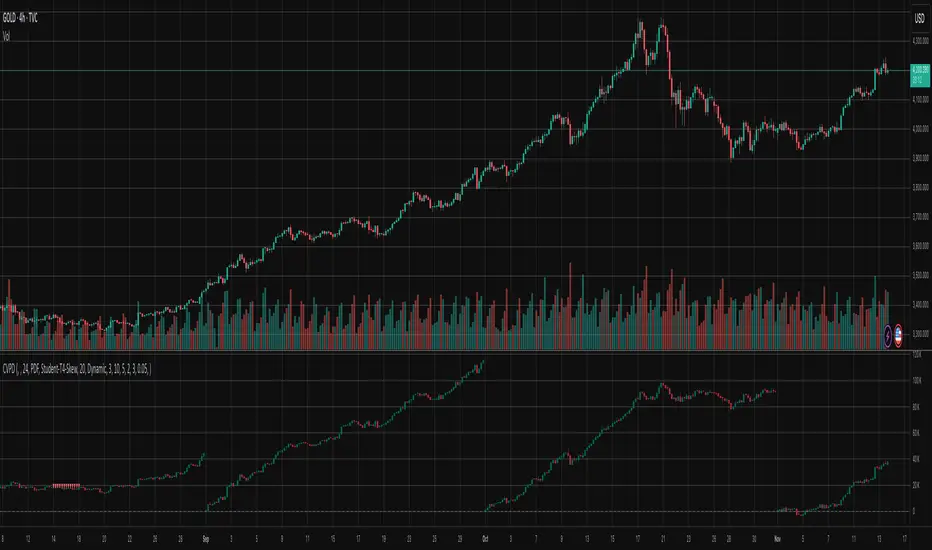
Cumulative Volume Profile DeltaThis indicator calculates the Cumulative Volume Profile Delta (CVPD). It constructs a high-resolution volume profile for each bar using intra-bar data, then derives and accumulates the delta from that profile to show net buying/selling pressure.
Key Features:
Statistical Volume Profile Engine: For each bar, the indicator builds a high-resolution volume profile on a lower 'Intra-Bar Timeframe'. Instead of simple tick counting, it uses statistical models ('PDF' allocation) to distribute volume across price levels and advanced classifiers ('Dynamic' split) to determine the buy/sell pressure before accumulation.
Periodic Accumulation: The CVPD accumulation is anchored to a user-defined 'Anchor Timeframe' (e.g., daily, weekly). This cyclical reset allows to analyze the build-up of pressure within specific trading periods.
"Delta Candle" Visualization: The periodic CVPD is shown as a candle, where:
Open: The CVPD value at the start of the period (or zero).
High/Low: Represent the peak buying (CVD High) and selling (CVD Low) pressure within that period's profile.
Close: The final net delta value (CVD) for the period.
Dual CVD & Divergence Engine: The indicator calculates two CVPDs: a Periodic one (for plotting) and a Continuous one (non-resetting). The continuous line is used as a stable source for the built-in divergence engine (detecting Regular, Hidden, and Exaggerated).
Dynamic Divergence Plotting: Divergence markers are plotted relative to the periodic (candle) CVPD. They automatically adjust their vertical position after a reset to remain visually aligned with the plotted candles.
Note on Confirmation (Lag): Divergence signals rely on a pivot confirmation method to ensure they do not repaint.
The Start of a- divergence is only detected after the confirming pivot is fully formed (a delay based on Pivot Right Bars).
The End of a divergence is detected either instantly (if the signal is invalidated by price action) or with a delay (when a new, non-divergent pivot is confirmed).
Multi-Timeframe (MTF) Capability:
MTF Output: The entire analysis (Delta Candles, Divergences) can be calculated on a higher timeframe (using the Timeframe input), with standard options to handle gaps (Fill Gaps) and prevent repainting (Wait for...).
Limitation: The Divergence detection engine (pivDiv) is disabled if a Higher Timeframe (HTF) is selected.
Integrated Alerts: Includes 18 comprehensive alerts for:
The start and end of all 6 divergence types.
The periodic CVPD crossing the zero line.
Conditions of agreement or disagreement between the delta and the main bar's direction.
Caution: Real-Time Data Behavior (Intra-Bar Repainting) This indicator uses high-resolution intra-bar data. As a result, the values on the current, unclosed bar (the real-time bar) will update dynamically as new intra-bar data arrives. This behavior is normal and necessary for this type of analysis. Signals should only be considered final after the main chart bar has closed.
DISCLAIMER
For Informational/Educational Use Only: This indicator is provided for informational and educational purposes only. It does not constitute financial, investment, or trading advice, nor is it a recommendation to buy or sell any asset.
Use at Your Own Risk: All trading decisions you make based on the information or signals generated by this indicator are made solely at your own risk.
No Guarantee of Performance: Past performance is not an indicator of future results. The author makes no guarantee regarding the accuracy of the signals or future profitability.
No Liability: The author shall not be held liable for any financial losses or damages incurred directly or indirectly from the use of this indicator.
Signals Are Not Recommendations: The alerts and visual signals (e.Example: crossovers) generated by this tool are not direct recommendations to buy or sell. They are technical observations for your own analysis and consideration.
Volume Profile DeltaThis indicator calculates the Volume Profile Delta (VPD). It constructs a high-resolution volume profile for each bar using intra-bar data, offering a detailed understanding of buying and selling pressure at discrete price levels.
Key Features:
Statistical Volume Profile Engine: For each bar, the indicator builds a high-resolution volume profile on a lower 'Intra-Bar Timeframe'. Instead of simple tick counting, it uses statistical models ('PDF' allocation) to distribute volume across price levels and advanced classifiers ('Dynamic' split) to determine the buy/sell pressure within that profile, providing a more nuanced delta calculation.
"Delta Candle" Visualization: The per-bar VPD is displayed as a candle, where:
Open: Always anchored at the zero line.
High/Low: Represent the peak buying (CVD High) and selling (CVD Low) pressure accumulated within that bar's profile.
Close: The final net delta value (CVD) for the bar.
Customizable Moving Average: An optional moving average of the net delta (Close) can be added. The MA type, length, and an optional Volume weighted setting are customizable.
Intra-Bar Peak Pivot Detection: Automatically identifies and plots significant turning points (pivots) in the peak buying (High) and selling (Low) pressure.
Note on Confirmation (Lag): Pivot signals are confirmed using a lookback method. A pivot is only plotted after the Pivot Right Bars input has passed, which introduces an inherent lag.
Multi-Timeframe (MTF) Capability:
MTF Output: The entire analysis (Delta Candles, MA, Pivots) can be calculated on a higher timeframe (using the Timeframe input), with standard options to handle gaps (Fill Gaps) and prevent repainting (Wait for...).
Limitation: The Pivot detection (Calculate Pivots) is disabled if a Higher Timeframe (HTF) is selected.
Integrated Alerts: Includes 8 alerts for:
The net delta crossing its moving average.
The detection of new peak buying or selling pivots.
Conditions of agreement or disagreement between the net delta and the main bar's direction.
Caution: Real-Time Data Behavior (Intra-Bar Repainting) This indicator uses high-resolution intra-bar data. As a result, the values on the current, unclosed bar (the real-time bar) will update dynamically as new intra-bar data arrives. This behavior is normal and necessary for this type of analysis. Signals should only be considered final after the main chart bar has closed.
DISCLAIMER
For Informational/Educational Use Only: This indicator is provided for informational and educational purposes only. It does not constitute financial, investment, or trading advice, nor is it a recommendation to buy or sell any asset.
Use at Your Own Risk: All trading decisions you make based on the information or signals generated by this indicator are made solely at your own risk.
No Guarantee of Performance: Past performance is not an indicator of future results. The author makes no guarantee regarding the accuracy of the signals or future profitability.
No Liability: The author shall not be held liable for any financial losses or damages incurred directly or indirectly from the use of this indicator.
Signals Are Not Recommendations: The alerts and visual signals (e.g., crossovers) generated by this tool are not direct recommendations to buy or sell. They are technical observations for your own analysis and consideration.

EMA Oscillator [Alpha Extract]A precision mean reversion analysis tool that combines advanced Z-score methodology with dual threshold systems to identify extreme price deviations from trend equilibrium. Utilizing sophisticated statistical normalization and adaptive percentage-based thresholds, this indicator provides high-probability reversal signals based on standard deviation analysis and dynamic range calculations with institutional-grade accuracy for systematic counter-trend trading opportunities.
🔶 Advanced Statistical Normalization
Calculates normalized distance between price and exponential moving average using rolling standard deviation methodology for consistent interpretation across timeframes. The system applies Z-score transformation to quantify price displacement significance, ensuring statistical validity regardless of market volatility conditions.
// Core EMA and Oscillator Calculation
ema_values = ta.ema(close, ema_period)
oscillator_values = close - ema_values
rolling_std = ta.stdev(oscillator_values, ema_period)
z_score = oscillator_values / rolling_std
🔶 Dual Threshold System
Implements both statistical significance thresholds (±1σ, ±2σ, ±3σ) and percentage-based dynamic thresholds calculated from recent oscillator range extremes. This hybrid approach ensures consistent probability-based signals while adapting to varying market volatility regimes and maintaining signal relevance during structural market changes.
// Statistical Thresholds
mild_threshold = 1.0 // ±1σ (68% confidence)
moderate_threshold = 2.0 // ±2σ (95% confidence)
extreme_threshold = 3.0 // ±3σ (99.7% confidence)
// Percentage-Based Dynamic Thresholds
osc_high = ta.highest(math.abs(z_score), lookback_period)
mild_pct_thresh = osc_high * (mild_pct / 100.0)
moderate_pct_thresh = osc_high * (moderate_pct / 100.0)
extreme_pct_thresh = osc_high * (extreme_pct / 100.0)
🔶 Signal Generation Framework
Triggers buy/sell alerts when Z-score crosses extreme threshold boundaries, indicating statistically significant price deviations with high mean reversion probability. The system generates continuation signals at moderate levels and reversal signals at extreme boundaries with comprehensive alert integration.
// Extreme Signal Detection
sell_signal = ta.crossover(z_score, selected_extreme)
buy_signal = ta.crossunder(z_score, -selected_extreme)
// Dynamic Color Coding
signal_color = z_score >= selected_extreme ? #ff0303 : // Extremely Overbought
z_score >= selected_moderate ? #ff6a6a : // Overbought
z_score >= selected_mild ? #b86456 : // Mildly Overbought
z_score > -selected_mild ? #a1a1a1 : // Neutral
z_score > -selected_moderate ? #01b844 : // Mildly Oversold
z_score > -selected_extreme ? #00ff66 : // Oversold
#00ff66 // Extremely Oversold
🔶 Visual Structure Analysis
Provides a six-tier color gradient system with dynamic background zones indicating mild, moderate, and extreme conditions. The histogram visualization displays Z-score intensity with threshold reference lines and zero-line equilibrium context for precise mean reversion timing.
snapshot
4H
1D
🔶 Adaptive Threshold Selection
Features intelligent threshold switching between statistical significance levels and percentage-based dynamic ranges. The percentage system automatically adjusts to current volatility conditions using configurable lookback periods, while statistical thresholds maintain consistent probability-based signal generation across market cycles.
🔶 Performance Optimization
Utilizes efficient rolling calculations with configurable EMA periods and threshold parameters for optimal performance across all timeframes. The system includes comprehensive alert functionality with customizable notification preferences and visual signal overlay options.
🔶 Market Oscillator Interpretation
Z-score > +3σ indicates statistically significant overbought conditions with high reversal probability, while Z-score < -3σ signals extreme oversold levels suitable for counter-trend entries. Moderate thresholds (±2σ) capture 95% of normal price distributions, making breaches statistically significant for systematic trading approaches.
snapshot
🔶 Intelligent Signal Management
Automatic signal filtering prevents false alerts through extreme threshold crossover requirements, while maintaining sensitivity to genuine statistical deviations. The dual threshold system provides both conservative statistical approaches and adaptive market condition responses for varying trading styles.
Why Choose EMA Oscillator ?
This indicator provides traders with statistically-grounded mean reversion analysis through sophisticated Z-score normalization methodology. By combining traditional statistical significance thresholds with adaptive percentage-based extremes, it maintains effectiveness across varying market conditions while delivering high-probability reversal signals based on quantifiable price displacement from trend equilibrium, enabling systematic counter-trend trading approaches with defined statistical confidence levels and comprehensive risk management parameters.

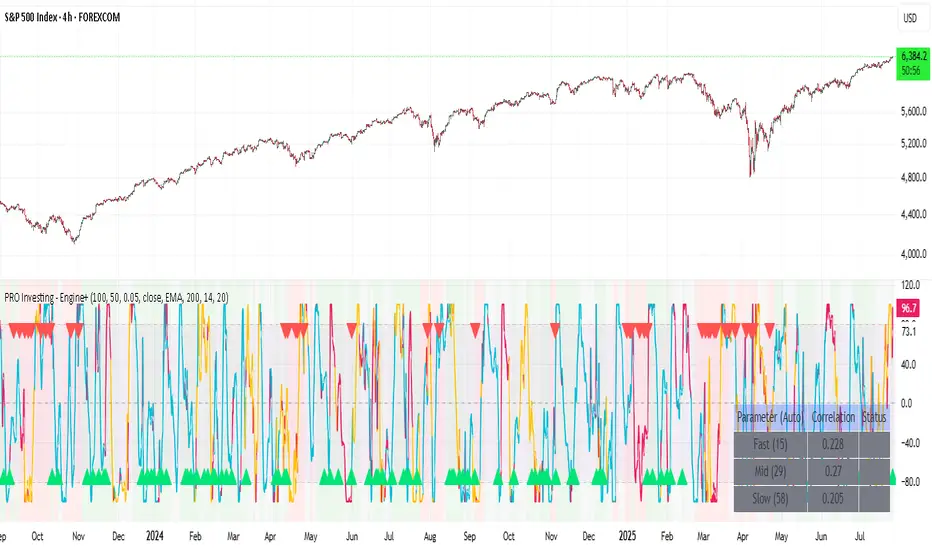
PRO Investing - Apex EnginePRO Investing - Apex Engine
1. Core Concept: Why Does This Indicator Exist?
Traditional momentum oscillators like RSI or Stochastic use a fixed "lookback period" (e.g., 14). This creates a fundamental problem: a 14-period setting that works well in a fast, trending market will generate constant false signals in a slow, choppy market, and vice-versa. The market's character is dynamic, but most tools are static.
The Apex Engine was built to solve this problem. Its primary innovation is a self-optimizing core that continuously adapts to changing market conditions. Instead of relying on one fixed setting, it actively tests three different momentum profiles (Fast, Mid, and Slow) in real-time and selects the one that is most synchronized with the current price action.
This is not just a random combination of indicators; it's a deliberate synthesis designed to create a more robust momentum tool. It combines:
Volatility analysis (ATR) to generate adaptive lookback periods.
Momentum measurement (ROC) to gauge the speed of price changes.
Statistical analysis (Correlation) to validate which momentum measurement is most effective right now.
Classic trend filters (Moving Average, ADX) to ensure signals are only taken in favorable market conditions.
The result is an oscillator that aims to be more responsive in volatile trends and more stable in quiet periods, providing a more intelligent and adaptive signal.
2. How It Works: The Engine's Three-Stage Process
To be transparent, it's important to understand the step-by-step logic the indicator follows on every bar. It's a process of Adapt -> Validate -> Signal.
Stage 1: Adapt (Dynamic Length Calculation)
The engine first measures market volatility using the Average True Range (ATR) relative to its own long-term average. This creates a volatility_factor. In high-volatility environments, this factor causes the base calculation lengths to shorten. In low-volatility, they lengthen. This produces three potential Rate of Change (ROC) lengths: dynamic_fast_len, dynamic_mid_len, and dynamic_slow_len.
Stage 2: Validate (Self-Optimizing Mode Selection)
This is the core of the engine. It calculates the ROC for all three dynamic lengths. To determine which is best, it uses the ta.correlation() function to measure how well each ROC's movement has correlated with the actual bar-to-bar price changes over the "Optimization Lookback" period. The ROC length with the highest correlation score is chosen as the most effective profile for the current moment. This "active" mode is reflected in the oscillator's color and the dashboard.
Stage 3: Signal (Normalized Velocity Oscillator)
The winning ROC series is then normalized into a consistent oscillator (the Velocity line) that ranges from -100 (extreme oversold) to +100 (extreme overbought). This ensures signals are comparable across any asset or timeframe. Signals are only generated when this Velocity line crosses its signal line and the trend filters (explained below) give a green light.
3. How to Use the Indicator: A Practical Guide
Reading the Visuals:
Velocity Line (Blue/Yellow/Pink): The main oscillator line. Its color indicates which mode is active (Fast, Mid, or Slow).
Signal Line (White): A moving average of the Velocity line. Crossovers generate potential signals.
Buy/Sell Triangles (▲ / ▼): These are your primary entry signals. They are intentionally strict and only appear when momentum, trend, and price action align.
Background Color (Green/Red/Gray): This is your trend context.
Green: Bullish trend confirmed (e.g., price above a rising 200 EMA and ADX > 20). Only Buy signals (▲) can appear.
Red: Bearish trend confirmed. Only Sell signals (▼) can appear.
Gray: No clear trend. The market is likely choppy or consolidating. No signals will appear; it is best to stay out.
Trading Strategy Example:
Wait for a colored background. A green or red background indicates the market is in a tradable trend.
Look for a signal. For a green background, wait for a lime Buy triangle (▲) to appear.
Confirm the trade. Before entering, confirm the signal aligns with your own analysis (e.g., support/resistance levels, chart patterns).
Manage the trade. Set a stop-loss according to your risk management rules. An exit can be considered on a fixed target, a trailing stop, or when an opposing signal appears.
4. Settings and Customization
This script is open-source, and its settings are transparent. You are encouraged to understand them.
Synaptic Engine Group:
Volatility Period: The master control for the adaptive engine. Higher values are slower and more stable.
Optimization Lookback: How many bars to use for the correlation check.
Switch Sensitivity: A buffer to prevent frantic switching between modes.
Advanced Configuration & Filters Group:
Price Source: The data source for momentum calculation (default close).
Trend Filter MA Type & Length: Define your long-term trend.
Filter by MA Slope: A key feature. If ON, allows for "buy the dip" entries below a rising MA. If OFF, it's stricter, requiring price to be above the MA.
ADX Length & Threshold: Filters out non-trending, choppy markets. Signals will not fire if the ADX is below this threshold.
5. Important Disclaimer
This indicator is a decision-support tool for discretionary traders, not an automated trading system or financial advice. Past performance is not indicative of future results. All trading involves substantial risk. You should always use proper risk management, including setting stop-losses, and never risk more than you are prepared to lose. The signals generated by this script should be used as one component of a broader trading plan.
Adaptive Supply and Demand [EdgeTerminal]Adaptive Supply and Demand is a dynamic supply and demand indicator with a few unique twists. It considers volume pressure, volatility-based adjustments and multi-time frame momentum for confidence scoring (multi-step confirmation) to generate dynamic lines that adjust based on the market and also to generate dynamic support/resistance levels for the supply and demand lines.
The dynamic support and resistance lines shown gives you a better situational awareness of the current state of the market and add more context to why the market is moving into a certain direction.
> Trading Scenarios
When the confidence score is over 80%, strong volume pressure in trend direction (up or down), volatility is low and momentum is aligned across timeframes, there is an indication of a strong upward or downward trend.
When the supply and demand line crossover, the confidence score is over 75% and the volume pressure is shifting, this can be an indicator of trend reversal. Use tight initial stops, scale into position as trend develops, monitor the volume pressure for continuation and wait for confidence confirmation.
When the confiance score is below 60%, the volume pressure is choppy, volatility is high, you want to avoid trading or reduce position size, wait for confidence improvements, use support and resistance for entries/exits and use tighter stops due to market conditions. This is an indication of a ranging market.
Another scenario is when there is a sudden volume pressure increase, and a raising confidence score, the volatility is expanding and the bar momentum is aligning the volatility direction. This can indicate a breakout scenario.
> How it Works
1. Volume Pressure Analysis
Volume Pressure Analysis is a key component that measures the true buying and selling force in the market. Here's a detailed breakdown. The idea is to standardize volume to prevent large spikes from skewing results.
The indicator employs an adaptive volume normalization technique to detect genuine buying and selling pressure.
It takes current volume and divides it by average volume.
If normVol > 1: Current volume is above average
If normVol < 1: Current volume is below average
An example if this would be If current volume is 1500 and average is 1000, normVol = 1.5 (50% above average)
Another component of the volume pressure analysis is the Price Change Calculation sub-module. The purpose of this is to measure price movement relative to recent average.
It works by subtracting the average price from the current price. If the value is positive, price is average and if negative, price is below average.
Finally, the volume pressure is calculated to combine volume and price for true pressure reading.
2. Savitzky-Golay Filtering
SG filtering implements advanced signal smoothing while preserving important trend features. It uses weighted moving average approximation, preserves higher moments of data and reduces noise while maintaining signal integrity.
This results in smoother signal lines, reduced false crossovers and better trend identification. Traditional moving averages tend to lag and smooth out important features. Additionally, simple moving averages can miss critical turning points and regular smoothing can delay signal generation.
SG filtering preserves higher moments such as peaks, valleys and trends, reduces noise while maintaining signal sharpness.
It works by creating a symmetric weighting scheme. This way center points get the highest weights while edge points get the lowest weight.
3. Parkinson's Volatility
Parkinson's Volatility is an advanced volatility measurement formula using high-low range data. It uses high-low range for volatility calculation, incorporates logarithmic returns and annualized the volatility measure.
This results in more accurate volatility measurement, better risk assessment and dynamic signal sensitivity.
4. Multi-timeframe Momentum
This combines signals from each module for each timeframe to calculate momentum across three timeframes. It also applies weighted importance to each timeframe and generates a composite momentum signal.
This results in a more comprehensive trend analysis, reduced timeframe bias and better trend confirmation.
> Indicator Settings
Short-term Period:
Lower values makes it more sensitive, meaning it will generate more signals. Higher values makes it less sensitive, resulting in fewer signals. We recommend a 5 to 15 range for day trading, and 10 to 20 for swing trading
Medium-term Period:
Lower values result in faster trend confirmation and higher values show slower and more reliable confirmation. We recommend a range of 15-25 for day trading and 20-30 for swing trading.
Long-term Period:
Lower values makes it more responsive to trend changes and higher values are better for major trend identification. We recommend a range of 40-60 for day trading and 50-100 for swing trading.
Volume Analysis Window:
Lower values result in more sensitivity to volume changes and higher values result in smoother volume analysis. The optimal range is 15-25 for most trading styles.
Confidence Threshold:
Lower values generate more signals but quality decreases. Higher values generate fewer signals but accuracy increases.The optimal range is 0.65-0.8 for most trading conditions.

Moving Averages With Continuous Periods [macp]This script reimagines traditional moving averages by introducing floating-point period calculations, allowing for fractional lengths rather than being constrained to whole numbers. At its core, it provides SMA, WMA, and HMA variants that can work with any decimal length, which proves especially valuable when creating dynamic indicators or fine-tuning existing strategies.
The most significant improvement lies in the Hull Moving Average implementation. By properly handling floating-point mathematics throughout the calculation chain, this version reduces the overshoot tendencies that often plague integer-based HMAs. The result is a more responsive yet controlled indicator that better captures price action without excessive whipsaw.
The visual aspect incorporates a trend gradient system that can adapt to different trading styles. Rather than using fixed coloring, it offers several modes ranging from simple solid colors to more nuanced three-tone gradients that help identify trend transitions. These gradients are normalized against ATR to provide context-aware visual feedback about trend strength.
From a practical standpoint, the floating-point approach eliminates the subtle discontinuities that occur when integer-based moving averages switch periods. This makes the indicator particularly useful in systems where the MA period itself is calculated from market conditions, as it can smoothly transition between different lengths without artificial jumps.
At the heart of this implementation lies the concept of continuous weights rather than discrete summation. Traditional moving averages treat each period as a distinct unit with integer indexing. However, when we move to floating-point periods, we need to consider how fractional periods should behave. This leads us to some interesting mathematical considerations.
Consider the Weighted Moving Average kernel. The weight function is fundamentally a slope: -x + length where x represents the position in the averaging window. The normalization constant is calculated by integrating (in our discrete case, summing) this slope across the window. What makes this implementation special is how it handles the fractional component - when the length isn't a whole number, the final period gets weighted proportionally to its fractional part.
For the Hull Moving Average, the mathematics become particularly intriguing. The standard HMA formula HMA = WMA(2*WMA(price, n/2) - WMA(price, n), sqrt(n)) is preserved, but now each WMA calculation operates in continuous space. This creates a smoother cascade of weights that better preserves the original intent of the Hull design - to reduce lag while maintaining smoothness.
The Simple Moving Average's treatment of fractional periods is perhaps the most elegant. For a length like 9.7, it weights the first 9 periods fully and the 10th period at 0.7 of its value. This creates a natural transition between integer periods that traditional implementations miss entirely.
The Gradient Mathematics
The trend gradient system employs normalized angular calculations to determine color transitions. By taking the arctangent of price changes normalized by ATR, we create a bounded space between 0 and 1 that represents trend intensity. The formula (arctan(Δprice/ATR) + 90°)/180° maps trend angles to this normalized space, allowing for smooth color transitions that respect market volatility context.
This mathematical framework creates a more theoretically sound foundation for moving averages, one that better reflects the continuous nature of price movement in financial markets. The implementation recognizes that time in markets isn't truly discrete - our sampling might be, but the underlying process we're trying to measure is continuous. By allowing for fractional periods, we're creating a better approximation of this continuous reality.
This floating-point moving average implementation offers tangible benefits for traders and analysts who need precise control over their indicators. The ability to fine-tune periods and create smooth transitions makes it particularly valuable for automated systems where moving average lengths are dynamically calculated from market conditions. The Hull Moving Average calculation now accurately reflects its mathematical formula while maintaining responsiveness, making it a practical choice for both systematic and discretionary trading approaches. Whether you're building dynamic indicators, optimizing existing strategies, or simply want more precise control over your moving averages, this implementation provides the mathematical foundation to do so effectively.
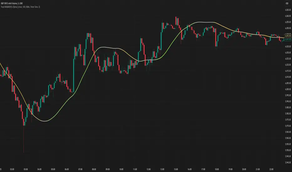
Watermark with dynamic variables [BM]█ OVERVIEW
This indicator allows users to add highly customizable watermark messages to their charts. Perfect for branding, annotation, or displaying dynamic chart information, this script offers advanced customization options including dynamic variables, text formatting, and flexible positioning.
█ CONCEPTS
Watermarks are overlay messages on charts. This script introduces placeholders — special keywords wrapped in % signs — that dynamically replace themselves with chart-related data. These watermarks can enhance charts with context, timestamps, or branding.
█ FEATURES
Dynamic Variables : Replace placeholders with real-time data such as bar index, timestamps, and more.
Advanced Customization : Modify text size, color, background, and alignment.
Multiple Messages : Add up to four independent messages per group, with two groups supported (A and B).
Positioning Options : Place watermarks anywhere on the chart using predefined locations.
Timezone Support : Display timestamps in a preferred timezone with customizable formats.
█ INPUTS
The script offers comprehensive input options for customization. Each Watermark (A and B) contains identical inputs for configuration.
Watermark settings are divided into two levels:
Watermark-Level Settings
These settings apply to the entire watermark group (A/B):
Show Watermark: Toggle the visibility of the watermark group on the chart.
Position: Choose where the watermark group is displayed on the chart.
Reverse Line Order: Enable to reverse the order of the lines displayed in Watermark A.
Message-Level Settings
Each watermark contains up to four configurable messages. These messages can be independently customized with the following options:
Message Content: Enter the custom text to be displayed. You can include placeholders for dynamic data.
Text Size: Select from predefined sizes (Tiny, Small, Normal, Large, Huge) or specify a custom size.
Text Alignment and Colors:
- Adjust the alignment of the text (Left, Center, Right).
- Set text and background colors for better visibility.
Format Time: Enable time formatting for this watermark message and configure the format and timezone. The settings for each message include message content, text size, alignment, and more. Please refer to Formatting dates and times for more details on valid formatting tokens.
█ PLACEHOLDERS
Placeholders are special keywords surrounded by % signs, which the script dynamically replaces with specific chart-related data. These placeholders allow users to insert dynamic content, such as bar information or timestamps, into watermark messages.
Below is the complete list of currently available placeholders:
bar_index , barstate.isconfirmed , barstate.isfirst , barstate.ishistory , barstate.islast , barstate.islastconfirmedhistory , barstate.isnew , barstate.isrealtime , chart.is_heikinashi , chart.is_kagi , chart.is_linebreak , chart.is_pnf , chart.is_range , chart.is_renko , chart.is_standard , chart.left_visible_bar_time , chart.right_visible_bar_time , close , dayofmonth , dayofweek , dividends.future_amount , dividends.future_ex_date , dividends.future_pay_date , earnings.future_eps , earnings.future_period_end_time , earnings.future_revenue , earnings.future_time , high , hl2 , hlc3 , hlcc4 , hour , last_bar_index , last_bar_time , low , minute , month , ohlc4 , open , second , session.isfirstbar , session.isfirstbar_regular , session.islastbar , session.islastbar_regular , session.ismarket , session.ispostmarket , session.ispremarket , syminfo.basecurrency , syminfo.country , syminfo.currency , syminfo.description , syminfo.employees , syminfo.expiration_date , syminfo.industry , syminfo.main_tickerid , syminfo.mincontract , syminfo.minmove , syminfo.mintick , syminfo.pointvalue , syminfo.prefix , syminfo.pricescale , syminfo.recommendations_buy , syminfo.recommendations_buy_strong , syminfo.recommendations_date , syminfo.recommendations_hold , syminfo.recommendations_sell , syminfo.recommendations_sell_strong , syminfo.recommendations_total , syminfo.root , syminfo.sector , syminfo.session , syminfo.shareholders , syminfo.shares_outstanding_float , syminfo.shares_outstanding_total , syminfo.target_price_average , syminfo.target_price_date , syminfo.target_price_estimates , syminfo.target_price_high , syminfo.target_price_low , syminfo.target_price_median , syminfo.ticker , syminfo.tickerid , syminfo.timezone , syminfo.type , syminfo.volumetype , ta.accdist , ta.iii , ta.nvi , ta.obv , ta.pvi , ta.pvt , ta.tr , ta.vwap , ta.wad , ta.wvad , time , time_close , time_tradingday , timeframe.isdaily , timeframe.isdwm , timeframe.isintraday , timeframe.isminutes , timeframe.ismonthly , timeframe.isseconds , timeframe.isticks , timeframe.isweekly , timeframe.main_period , timeframe.multiplier , timeframe.period , timenow , volume , weekofyear , year
█ HOW TO USE
1 — Add the Script:
Apply "Watermark with dynamic variables " to your chart from the TradingView platform.
2 — Configure Inputs:
Open the script settings by clicking the gear icon next to the script's name.
Customize visibility, message content, and appearance for Watermark A and Watermark B.
3 — Utilize Placeholders:
Add placeholders like %bar_index% or %timenow% in the "Watermark - Message" fields to display dynamic data.
Empty lines in the message box are reflected on the chart, allowing you to shift text up or down.
Using in the message box translates to a new line on the chart.
4 — Preview Changes:
Adjust settings and view updates in real-time on your chart.
█ EXAMPLES
Branding
DodgyDD's charts
Debugging
█ LIMITATIONS
Only supports variables defined within the script.
Limited to four messages per watermark.
Visual alignment may vary across different chart resolutions or zoom levels.
Placeholder parsing relies on correct input formatting.
█ NOTES
This script is designed for users seeking enhanced chart annotation capabilities. It provides tools for dynamic, customizable watermarks but is not a replacement for chart objects like text labels or drawings. Please ensure placeholders are properly formatted for correct parsing.
Additionally, this script can be a valuable tool for Pine Script developers during debugging . By utilizing dynamic placeholders, developers can display real-time values of variables and chart data directly on their charts, enabling easier troubleshooting and code validation.
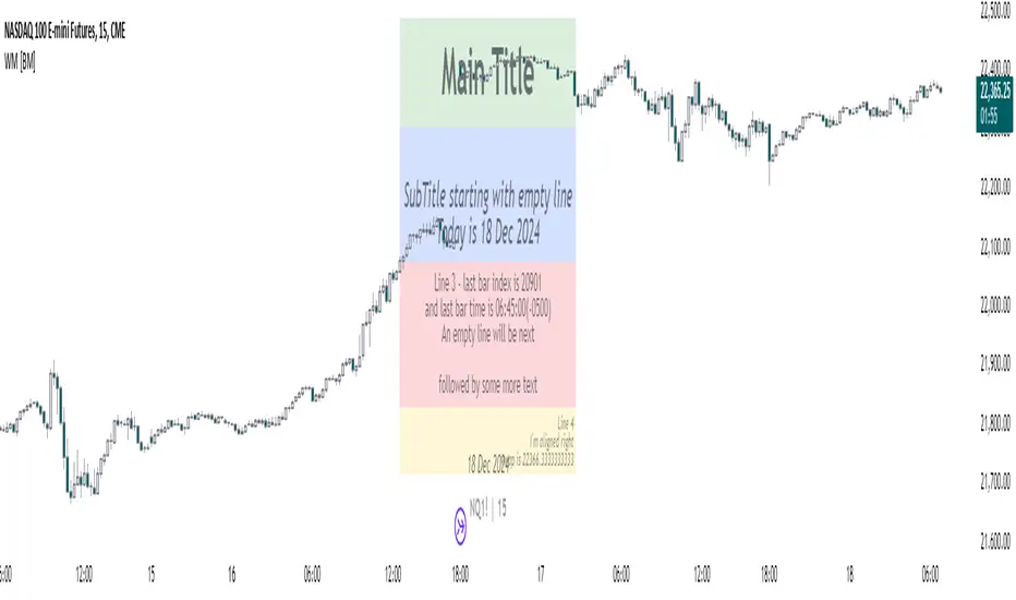
Hybrid Adaptive Double Exponential Smoothing🙏🏻 This is HADES (Hybrid Adaptive Double Exponential Smoothing) : fully data-driven & adaptive exponential smoothing method, that gains all the necessary info directly from data in the most natural way and needs no subjective parameters & no optimizations. It gets applied to data itself -> to fit residuals & one-point forecast errors, all at O(1) algo complexity. I designed it for streaming high-frequency univariate time series data, such as medical sensor readings, orderbook data, tick charts, requests generated by a backend, etc.
The HADES method is:
fit & forecast = a + b * (1 / alpha + T - 1)
T = 0 provides in-sample fit for the current datum, and T + n provides forecast for n datapoints.
y = input time series
a = y, if no previous data exists
b = 0, if no previous data exists
otherwise:
a = alpha * y + (1 - alpha) * a
b = alpha * (a - a ) + (1 - alpha) * b
alpha = 1 / sqrt(len * 4)
len = min(ceil(exp(1 / sig)), available data)
sig = sqrt(Absolute net change in y / Sum of absolute changes in y)
For the start datapoint when both numerator and denominator are zeros, we define 0 / 0 = 1
...
The same set of operations gets applied to the data first, then to resulting fit absolute residuals to build prediction interval, and finally to absolute forecasting errors (from one-point ahead forecast) to build forecasting interval:
prediction interval = data fit +- resoduals fit * k
forecasting interval = data opf +- errors fit * k
where k = multiplier regulating intervals width, and opf = one-point forecasts calculated at each time t
...
How-to:
0) Apply to your data where it makes sense, eg. tick data;
1) Use power transform to compensate for multiplicative behavior in case it's there;
2) If you have complete data or only the data you need, like the full history of adjusted close prices: go to the next step; otherwise, guided by your goal & analysis, adjust the 'start index' setting so the calculations will start from this point;
3) Use prediction interval to detect significant deviations from the process core & make decisions according to your strategy;
4) Use one-point forecast for nowcasting;
5) Use forecasting intervals to ~ understand where the next datapoints will emerge, given the data-generating process will stay the same & lack structural breaks.
I advise k = 1 or 1.5 or 4 depending on your goal, but 1 is the most natural one.
...
Why exponential smoothing at all? Why the double one? Why adaptive? Why not Holt's method?
1) It's O(1) algo complexity & recursive nature allows it to be applied in an online fashion to high-frequency streaming data; otherwise, it makes more sense to use other methods;
2) Double exponential smoothing ensures we are taking trends into account; also, in order to model more complex time series patterns such as seasonality, we need detrended data, and this method can be used to do it;
3) The goal of adaptivity is to eliminate the window size question, in cases where it doesn't make sense to use cumulative moving typical value;
4) Holt's method creates a certain interaction between level and trend components, so its results lack symmetry and similarity with other non-recursive methods such as quantile regression or linear regression. Instead, I decided to base my work on the original double exponential smoothing method published by Rob Brown in 1956, here's the original source , it's really hard to find it online. This cool dude is considered the one who've dropped exponential smoothing to open access for the first time🤘🏻
R&D; log & explanations
If you wanna read this, you gotta know, you're taking a great responsability for this long journey, and it gonna be one hell of a trip hehe
Machine learning, apprentissage automatique, машинное обучение, digital signal processing, statistical learning, data mining, deep learning, etc., etc., etc.: all these are just artificial categories created by the local population of this wonderful world, but what really separates entities globally in the Universe is solution complexity / algorithmic complexity.
In order to get the game a lil better, it's gonna be useful to read the HTES script description first. Secondly, let me guide you through the whole R&D; process.
To discover (not to invent) the fundamental universal principle of what exponential smoothing really IS, it required the review of the whole concept, understanding that many things don't add up and don't make much sense in currently available mainstream info, and building it all from the beginning while avoiding these very basic logical & implementation flaws.
Given a complete time t, and yet, always growing time series population that can't be logically separated into subpopulations, the very first question is, 'What amount of data do we need to utilize at time t?'. Two answers: 1 and all. You can't really gain much info from 1 datum, so go for the second answer: we need the whole dataset.
So, given the sequential & incremental nature of time series, the very first and basic thing we can do on the whole dataset is to calculate a cumulative , such as cumulative moving mean or cumulative moving median.
Now we need to extend this logic to exponential smoothing, which doesn't use dataset length info directly, but all cool it can be done via a formula that quantifies the relationship between alpha (smoothing parameter) and length. The popular formulas used in mainstream are:
alpha = 1 / length
alpha = 2 / (length + 1)
The funny part starts when you realize that Cumulative Exponential Moving Averages with these 2 alpha formulas Exactly match Cumulative Moving Average and Cumulative (Linearly) Weighted Moving Average, and the same logic goes on:
alpha = 3 / (length + 1.5) , matches Cumulative Weighted Moving Average with quadratic weights, and
alpha = 4 / (length + 2) , matches Cumulative Weighted Moving Average with cubic weghts, and so on...
It all just cries in your shoulder that we need to discover another, native length->alpha formula that leverages the recursive nature of exponential smoothing, because otherwise, it doesn't make sense to use it at all, since the usual CMA and CMWA can be computed incrementally at O(1) algo complexity just as exponential smoothing.
From now on I will not mention 'cumulative' or 'linearly weighted / weighted' anymore, it's gonna be implied all the time unless stated otherwise.
What we can do is to approach the thing logically and model the response with a little help from synthetic data, a sine wave would suffice. Then we can think of relationships: Based on algo complexity from lower to higher, we have this sequence: exponential smoothing @ O(1) -> parametric statistics (mean) @ O(n) -> non-parametric statistics (50th percentile / median) @ O(n log n). Based on Initial response from slow to fast: mean -> median Based on convergence with the real expected value from slow to fast: mean (infinitely approaches it) -> median (gets it quite fast).
Based on these inputs, we need to discover such a length->alpha formula so the resulting fit will have the slowest initial response out of all 3, and have the slowest convergence with expected value out of all 3. In order to do it, we need to have some non-linear transformer in our formula (like a square root) and a couple of factors to modify the response the way we need. I ended up with this formula to meet all our requirements:
alpha = sqrt(1 / length * 2) / 2
which simplifies to:
alpha = 1 / sqrt(len * 8)
^^ as you can see on the screenshot; where the red line is median, the blue line is the mean, and the purple line is exponential smoothing with the formulas you've just seen, we've met all the requirements.
Now we just have to do the same procedure to discover the length->alpha formula but for double exponential smoothing, which models trends as well, not just level as in single exponential smoothing. For this comparison, we need to use linear regression and quantile regression instead of the mean and median.
Quantile regression requires a non-closed form solution to be solved that you can't really implement in Pine Script, but that's ok, so I made the tests using Python & sklearn:
paste.pics
^^ on this screenshot, you can see the same relationship as on the previous screenshot, but now between the responses of quantile regression & linear regression.
I followed the same logic as before for designing alpha for double exponential smoothing (also considered the initial overshoots, but that's a little detail), and ended up with this formula:
alpha = sqrt(1 / length) / 2
which simplifies to:
alpha = 1 / sqrt(len * 4)
Btw, given the pattern you see in the resulting formulas for single and double exponential smoothing, if you ever want to do triple (not Holt & Winters) exponential smoothing, you'll need len * 2 , and just len * 1 for quadruple exponential smoothing. I hope that based on this sequence, you see the hint that Maybe 4 rounds is enough.
Now since we've dealt with the length->alpha formula, we can deal with the adaptivity part.
Logically, it doesn't make sense to use a slower-than-O(1) method to generate input for an O(1) method, so it must be something universal and minimalistic: something that will help us measure consistency in our data, yet something far away from statistics and close enough to topology.
There's one perfect entity that can help us, this is fractal efficiency. The way I define fractal efficiency can be checked at the very beginning of the post, what matters is that I add a square root to the formula that is not typically added.
As explained in the description of my metric QSFS , one of the reasons for SQRT-transformed values of fractal efficiency applied in moving window mode is because they start to closely resemble normal distribution, yet with support of (0, 1). Data with this interesting property (normally distributed yet with finite support) can be modeled with the beta distribution.
Another reason is, in infinitely expanding window mode, fractal efficiency of every time series that exhibits randomness tends to infinitely approach zero, sqrt-transform kind of partially neutralizes this effect.
Yet another reason is, the square root might better reflect the dimensional inefficiency or degree of fractal complexity, since it could balance the influence of extreme deviations from the net paths.
And finally, fractals exhibit power-law scaling -> measures like length, area, or volume scale in a non-linear way. Adding a square root acknowledges this intrinsic property, while connecting our metric with the nature of fractals.
---
I suspect that, given analogies and connections with other topics in geometry, topology, fractals and most importantly positive test results of the metric, it might be that the sqrt transform is the fundamental part of fractal efficiency that should be applied by default.
Now the last part of the ballet is to convert our fractal efficiency to length value. The part about inverse proportionality is obvious: high fractal efficiency aka high consistency -> lower window size, to utilize only the last data that contain brand new information that seems to be highly reliable since we have consistency in the first place.
The non-obvious part is now we need to neutralize the side effect created by previous sqrt transform: our length values are too low, and exponentiation is the perfect candidate to fix it since translating fractal efficiency into window sizes requires something non-linear to reflect the fractal dynamics. More importantly, using exp() was the last piece that let the metric shine, any other transformations & formulas alike I've tried always had some weird results on certain data.
That exp() in the len formula was the last piece that made it all work both on synthetic and on real data.
^^ a standalone script calculating optimal dynamic window size
Omg, THAT took time to write. Comment and/or text me if you need
...
"Versace Pip-Boy, I'm a young gun coming up with no bankroll" 👻
∞
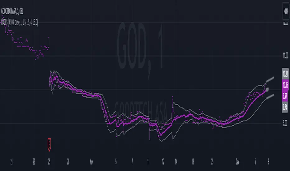
Adaptive Supertrend with Dynamic Optimization [EdgeTerminal]The Enhanced Adaptive Supertrend represents a significant evolution of the traditional Supertrend indicator, incorporating advanced mathematical optimization, dynamic volatility adjustment, intelligent signal filtering, reduced noise and false positives.
Key Features
Dynamic volatility-adjusted bands
Self-optimizing multiplier
Intelligent signal filtering system
Cooldown period to prevent signal clustering
Clear buy/sell signals with optimal positioning
Smooth trend visualization
RSI and MACD integration for confirmation
Performance-based optimization
Dynamic Band Calculation
Dynamic Band Calculation automatically adapts to market volatility, generates wider bands in volatile periods, reducing false signals. It also generates tighter bands in stable periods, capturing smaller moves and smooth transitions between different volatility regimes.
RSI Integration
The RSI and MACD play multiple crucial roles in the Adaptive Supertrend.
It first helps with momentum factor calculation. This dynamically adjusts band width based on momentum conditions. When the RSI is oversold, bands widen by 20% to prevent false signals during strong downtrends and provide more room for price movements in extreme conditions.
When the RSI is overbought, brands tighten by 20% and they become more sensitive to potential reversals to help catch trend changes earlier.
This reduces false signals in strong trends, helps detect potential reversals earlier than the usual, create adaptive band width based on market conditions and finally, better protection against whipsaws.
MACD Integration
The MACD in this supertrend indicator serves as a trend confirmation tool. The idea is to use MACD crossovers to confirm trend changes to reduce false trend change signals and enhance the signal quality.
For this to become a signal, MACD crossovers must align with price movement to help filter out weak or false signals, which acts as an additional layer of trend confirmation.
Additionally, MACD line position relative to signal line indicates trend strength, helps maintain positions in strong trends and assists in early detection of trend weakening.
Momentum Integration
Momentum Integration prevents false signals in extreme conditions, It adjusts dynamic bands based on market momentum, improves trend confirmation in strong moves and reduces whipsaws during consolidations.
Improved signals
There are a few systems to generate better signals, allowing for generally faster signals compared to original supertrend, such as:
Enforced cooldown period between signals
Prevents signal clustering
Clearer entry/exit points
Reduced false signals during choppy markets
Performance Optimization
This script implements a Sharpe ratio-inspired optimization algorithm to balance returns against risk, penalize large drawdowns, adapt parameters in real-time and improve risk-adjusted performance
Parameter Settings
ATR Period: 10 (default) - adjust based on timeframe
Initial Multiplier: 3.0 (default) - will self-optimize
Optimization Period: 50 (default) - longer periods for more stability
Smoothing Period: 3 (default) - adjust for signal smoothness
Best Practices
Use on multiple timeframes for confirmation
Allow the optimization process to run for at least 50 bars
Monitor the adaptive multiplier for trend strength indication
Consider RSI and MACD alignment for stronger signals
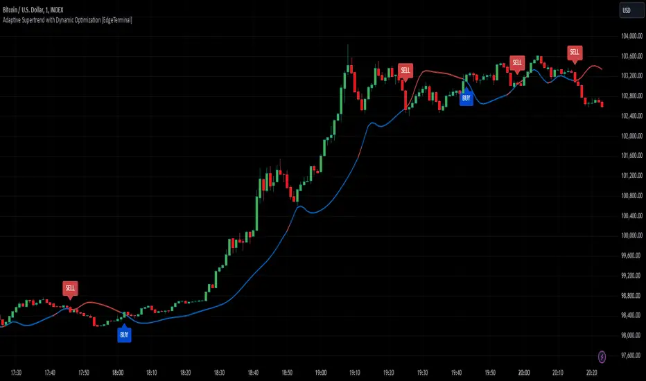
Dynamic Resistance and Support LinesThis script is designed to dynamically plot support and resistance lines based on full-dollar and half-dollar price levels relative to the close price on a chart. The script is particularly useful for day traders and scalpers, as it helps visualize key psychological price levels that often act as support and resistance zones in volatile and fast-moving markets in real time.
Key Features:
Dynamic Resistance and Support Levels:
Full-dollar levels: These are calculated by rounding the close price to the nearest full dollar and then extending the levels by adding and subtracting increments of 1 (e.g., $1, $2, $3).
Half-dollar levels: These are calculated by adding and subtracting 0.5 increments to the nearest full-dollar price, providing additional reference points. The historical full-dollar levels remain where support and resistance may have occurred in the past.
Extend Lines:
You can toggle whether the support and resistance lines are extended to the right, left, or both directions. This allows flexibility in projecting potential future areas of support or resistance.
Custom Line Extension:
The user can set the number of bars (or time periods) that the support and resistance lines will extend, giving control over how long the levels remain on the chart.
Color-Coded Lines:
Red lines represent full-dollar resistance and support levels.
Blue lines represent half-dollar levels, making it easy to differentiate between key psychological price zones.
Line Flexibility:
The script allows the lines to extend both left and right on the chart, making it useful for analyzing historical price action or projecting future price movements. The number of bars for extension is customizable, allowing for tailored setups.
Nearest Full Dollar Plot:
The nearest full-dollar price level is plotted as a yellow circle on the chart. This serves as a quick visual cue for traders to monitor price proximity to critical levels.
Benefits in Day Trading, Scalping, and Volatile Markets:
Visualizing Key Psychological Levels:
Full-dollar and half-dollar price levels often act as psychological barriers for traders. This script helps traders easily identify these levels, which are important in both fast-moving markets and during sideways consolidation.
Improved Decision-Making:
By automatically drawing these support and resistance levels, the script helps day traders and scalpers make quicker and more informed decisions, especially in volatile markets where every second counts.
Adaptability to Market Conditions:
The flexibility of extending lines based on trader preferences allows the user to adapt the script to various market conditions, such as high volatility or trend-based trading, providing a clear view of potential breakout or reversal areas.
Better Risk Management:
Having predefined support and resistance levels helps traders better manage risk, as these levels can act as logical areas for setting stop losses or taking profits.
This script is especially valuable for traders looking to capitalize on quick market movements or identify key entry and exit points during market volatility.
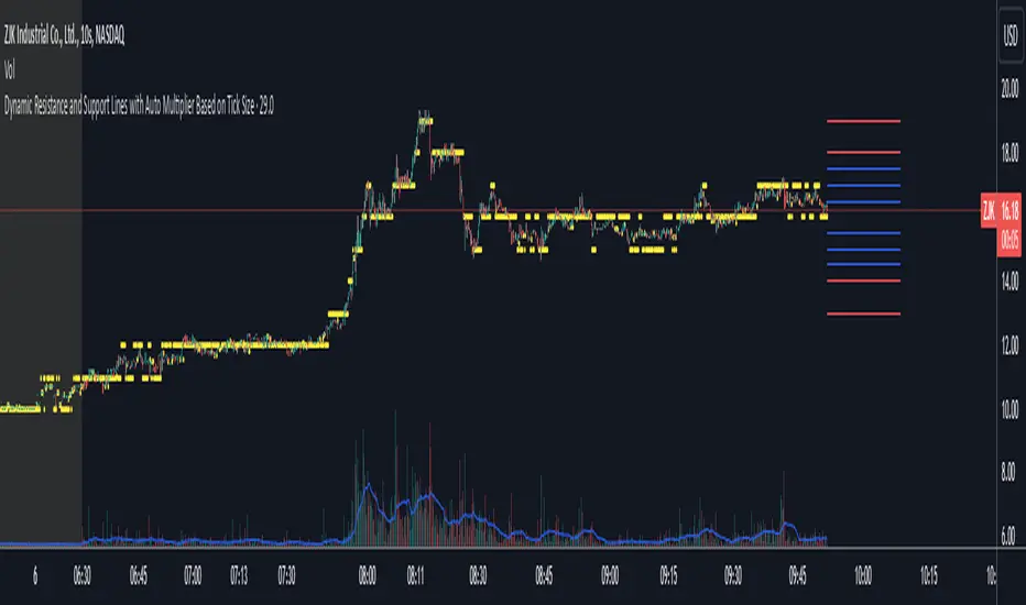
Dynamic Jurik RSX w/ Fisher Transform█ Introduction
The Dynamic Jurik RSX with Fisher Transform is a powerful and adaptive momentum indicator designed for traders who seek a non-laggy view of price movements. This script is based on the classic Jurik RSX (Relative Strength Index). It also includes features such as the dynamic overbought and oversold limits, the Inverse Fisher Transform, trend display, slope calculations, and the ability to color extremes for better clarity.
█ Key Features:
• RSX: The Relative Strength Index (RSX) in this script is based on Jurik’s RSX, which is smoother than the traditional RSI and aims to reduce noise and lag. This script calculates the RSX using an exponential smoothing technique and adaptive adjustments.
• Inverse Fisher Transform: This script can optionally apply the Inverse Fisher Transform to the RSX, which helps to normalize the RSX values, compressing them between -1 and 1. The inverse transformation makes it easier to spot extreme values (overbought and oversold conditions) by enhancing the visual clarity of those extremes. It also smooths the curve over a user-defined period in hopes of providing a more consistent signal.
• Dynamic Limits: The dynamic overbought and oversold limits are calculated based on the RSX's recent high and low values. The limits adjust dynamically depending on market conditions, making them more relevant to current price action.
• Slope Display: The slope of the RSX is calculated as the rate of change between the current and previous RSX value. The slope is displayed as dots when the slope exceeds the threshold designated by the user, providing visual cues for momentum shifts.
• Trend Coloring: Optionally, the user can also enable a trend-based display. It is simply based on current value of RSX versus the previous one. If RSX is rising then the trend is bullish, if not, then the trend is bearish.
• Coloring Extremes: Users can configure the RSX to color the chart when prices enter extreme conditions, such as overbought or oversold zones, providing visual cues for market reversals.
█ Attached Chart Notes:
• Top Panel: Enabled dynamic limits, Trend display, standard Jurik RSX with 20 lookback period, and Slope display.
• Middle Panel: Enabled dynamic limits, Extremes display, and standard Jurik RSX with 20 lookback period.
• Bottom Panel: Enabled dynamic limits, Trend display, Inverse Fisher Transform with 14 lookback period and 9 smoothing period. and Slope display.
█ Credits:
Special thanks to Everget for providing the original script. The script was also slightly modified based on updates from outside sources.
█ Disclaimer:
This script is for educational purposes only and should not be considered financial advice. Always conduct your own research and consult a professional before making any trading decisions.

Support Resistance UltimateThe "Support Resistance ULTIMATE" indicator is a comprehensive tool for traders on the TradingView platform, designed to identify key support and resistance levels using two primary techniques: pivot points and volume data. This indicator provides flexibility and customization, allowing traders to adapt it to their specific trading strategies.
KEY FEATURES
Pivot-Based Levels:
This feature calculates support and resistance levels using pivot points, which are derived from the high, low, and close prices of previous trading periods. Pivot points are crucial for forecasting potential market turning points.
Users can customize the pivot calculation by selecting the source type (either 'Close' or 'High/Low') and adjusting the lookback periods for both the left and right sides of the pivot calculation. This flexibility allows traders to adapt the indicator to different market conditions and timeframes.
Volume-Based Levels:
This option focuses on identifying support and resistance levels based on volume data, specifically the Point of Control (POC). The POC represents the price level with the highest traded volume during a specific time period, reflecting a consensus value among market participants.
The indicator includes a rolling POC calculation, allowing traders to dynamically assess areas of significant trading interest that may serve as support or resistance zones.
ADVANTAGES
Customization and Flexibility:
Traders can choose between pivot-based and volume-based levels or use both simultaneously, depending on their analysis needs. This dual approach provides a comprehensive view of market dynamics, accommodating various trading styles.
The indicator offers customizable color settings for support and resistance lines, enhancing chart readability and allowing traders to personalize their visual analysis.
Enhanced Market Insights:
By utilizing pivot points, traders can identify potential reversal or consolidation points, aiding in the prediction of market trends and the establishment of strategic entry and exit points.
Volume-based levels provide insights into market sentiment and participation, highlighting areas of strong support or resistance based on trading volume. This can improve risk management and trade execution by identifying high-probability trading zones.
Importance Scoring:
The indicator calculates the importance of each level based on the number of touches and the duration it holds. This scoring system helps traders assess the strength of support and resistance levels, with thicker lines indicating more significant levels.
This indicator is intended for educational and informational purposes only and should not be considered financial advice. Trading involves significant risk, and you should consult with a financial advisor before making any trading decisions. The performance of this indicator is not guaranteed, and past results do not predict future performance. Use at your own risk.