PINE LIBRARY
업데이트됨 FunctionBaumWelch
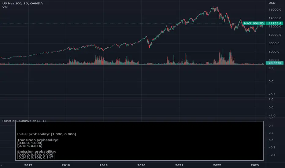
Library "FunctionBaumWelch"
Baum-Welch Algorithm, also known as Forward-Backward Algorithm, uses the well known EM algorithm
to find the maximum likelihood estimate of the parameters of a hidden Markov model given a set of observed
feature vectors.
---
### Function List:
> `forward (array<float> pi, matrix<float> a, matrix<float> b, array<int> obs)`
> `forward (array<float> pi, matrix<float> a, matrix<float> b, array<int> obs, bool scaling)`
> `backward (matrix<float> a, matrix<float> b, array<int> obs)`
> `backward (matrix<float> a, matrix<float> b, array<int> obs, array<float> c)`
> `baumwelch (array<int> observations, int nstates)`
> `baumwelch (array<int> observations, array<float> pi, matrix<float> a, matrix<float> b)`
---
### Reference:
> en.wikipedia.org/wiki/Baum–Welch_algorithm
> github.com/alexsosn/MarslandMLAlgo/blob/4277b24db88c4cb70d6b249921c5d21bc8f86eb4/Ch16/HMM.py
> en.wikipedia.org/wiki/Forward_algorithm
> rdocumentation.org/packages/HMM/versions/1.0.1/topics/forward
> rdocumentation.org/packages/HMM/versions/1.0.1/topics/backward
forward(pi, a, b, obs)
Computes forward probabilities for state `X` up to observation at time `k`, is defined as the
probability of observing sequence of observations `e_1 ... e_k` and that the state at time `k` is `X`.
Parameters:
pi (float[]): Initial probabilities.
a (matrix<float>): Transmissions, hidden transition matrix a or alpha = transition probability matrix of changing
states given a state matrix is size (M x M) where M is number of states.
b (matrix<float>): Emissions, matrix of observation probabilities b or beta = observation probabilities. Given
state matrix is size (M x O) where M is number of states and O is number of different
possible observations.
obs (int[]): List with actual state observation data.
Returns: - `matrix<float> _alpha`: Forward probabilities. The probabilities are given on a logarithmic scale (natural logarithm). The first
dimension refers to the state and the second dimension to time.
forward(pi, a, b, obs, scaling)
Computes forward probabilities for state `X` up to observation at time `k`, is defined as the
probability of observing sequence of observations `e_1 ... e_k` and that the state at time `k` is `X`.
Parameters:
pi (float[]): Initial probabilities.
a (matrix<float>): Transmissions, hidden transition matrix a or alpha = transition probability matrix of changing
states given a state matrix is size (M x M) where M is number of states.
b (matrix<float>): Emissions, matrix of observation probabilities b or beta = observation probabilities. Given
state matrix is size (M x O) where M is number of states and O is number of different
possible observations.
obs (int[]): List with actual state observation data.
scaling (bool): Normalize `alpha` scale.
Returns: - #### Tuple with:
> - `matrix<float> _alpha`: Forward probabilities. The probabilities are given on a logarithmic scale (natural logarithm). The first
dimension refers to the state and the second dimension to time.
> - `array<float> _c`: Array with normalization scale.
backward(a, b, obs)
Computes backward probabilities for state `X` and observation at time `k`, is defined as the probability of observing the sequence of observations `e_k+1, ... , e_n` under the condition that the state at time `k` is `X`.
Parameters:
a (matrix<float>): Transmissions, hidden transition matrix a or alpha = transition probability matrix of changing states
given a state matrix is size (M x M) where M is number of states
b (matrix<float>): Emissions, matrix of observation probabilities b or beta = observation probabilities. given state
matrix is size (M x O) where M is number of states and O is number of different possible observations
obs (int[]): Array with actual state observation data.
Returns: - `matrix<float> _beta`: Backward probabilities. The probabilities are given on a logarithmic scale (natural logarithm). The first dimension refers to the state and the second dimension to time.
backward(a, b, obs, c)
Computes backward probabilities for state `X` and observation at time `k`, is defined as the probability of observing the sequence of observations `e_k+1, ... , e_n` under the condition that the state at time `k` is `X`.
Parameters:
a (matrix<float>): Transmissions, hidden transition matrix a or alpha = transition probability matrix of changing states
given a state matrix is size (M x M) where M is number of states
b (matrix<float>): Emissions, matrix of observation probabilities b or beta = observation probabilities. given state
matrix is size (M x O) where M is number of states and O is number of different possible observations
obs (int[]): Array with actual state observation data.
c (float[]): Array with Normalization scaling coefficients.
Returns: - `matrix<float> _beta`: Backward probabilities. The probabilities are given on a logarithmic scale (natural logarithm). The first dimension refers to the state and the second dimension to time.
baumwelch(observations, nstates)
**(Random Initialization)** Baum–Welch algorithm is a special case of the expectation–maximization algorithm used to find the
unknown parameters of a hidden Markov model (HMM). It makes use of the forward-backward algorithm
to compute the statistics for the expectation step.
Parameters:
observations (int[]): List of observed states.
nstates (int)
Returns: - #### Tuple with:
> - `array<float> _pi`: Initial probability distribution.
> - `matrix<float> _a`: Transition probability matrix.
> - `matrix<float> _b`: Emission probability matrix.
---
requires: `import RicardoSantos/WIPTensor/2 as Tensor`
baumwelch(observations, pi, a, b)
Baum–Welch algorithm is a special case of the expectation–maximization algorithm used to find the
unknown parameters of a hidden Markov model (HMM). It makes use of the forward-backward algorithm
to compute the statistics for the expectation step.
Parameters:
observations (int[]): List of observed states.
pi (float[]): Initial probaility distribution.
a (matrix<float>): Transmissions, hidden transition matrix a or alpha = transition probability matrix of changing states
given a state matrix is size (M x M) where M is number of states
b (matrix<float>): Emissions, matrix of observation probabilities b or beta = observation probabilities. given state
matrix is size (M x O) where M is number of states and O is number of different possible observations
Returns: - #### Tuple with:
> - `array<float> _pi`: Initial probability distribution.
> - `matrix<float> _a`: Transition probability matrix.
> - `matrix<float> _b`: Emission probability matrix.
---
requires: `import RicardoSantos/WIPTensor/2 as Tensor`
릴리즈 노트
v2 minor update.릴리즈 노트
Fix logger version.릴리즈 노트
v4 - Added error checking for some errors.릴리즈 노트
v5 - Improved calculation by merging some of the loops, where possible.파인 라이브러리
트레이딩뷰의 진정한 정신에 따라, 작성자는 이 파인 코드를 오픈소스 라이브러리로 게시하여 커뮤니티의 다른 파인 프로그래머들이 재사용할 수 있도록 했습니다. 작성자에게 경의를 표합니다! 이 라이브러리는 개인적으로 사용하거나 다른 오픈소스 게시물에서 사용할 수 있지만, 이 코드의 게시물 내 재사용은 하우스 룰에 따라 규제됩니다.
면책사항
해당 정보와 게시물은 금융, 투자, 트레이딩 또는 기타 유형의 조언이나 권장 사항으로 간주되지 않으며, 트레이딩뷰에서 제공하거나 보증하는 것이 아닙니다. 자세한 내용은 이용 약관을 참조하세요.
파인 라이브러리
트레이딩뷰의 진정한 정신에 따라, 작성자는 이 파인 코드를 오픈소스 라이브러리로 게시하여 커뮤니티의 다른 파인 프로그래머들이 재사용할 수 있도록 했습니다. 작성자에게 경의를 표합니다! 이 라이브러리는 개인적으로 사용하거나 다른 오픈소스 게시물에서 사용할 수 있지만, 이 코드의 게시물 내 재사용은 하우스 룰에 따라 규제됩니다.
면책사항
해당 정보와 게시물은 금융, 투자, 트레이딩 또는 기타 유형의 조언이나 권장 사항으로 간주되지 않으며, 트레이딩뷰에서 제공하거나 보증하는 것이 아닙니다. 자세한 내용은 이용 약관을 참조하세요.