OPEN-SOURCE SCRIPT
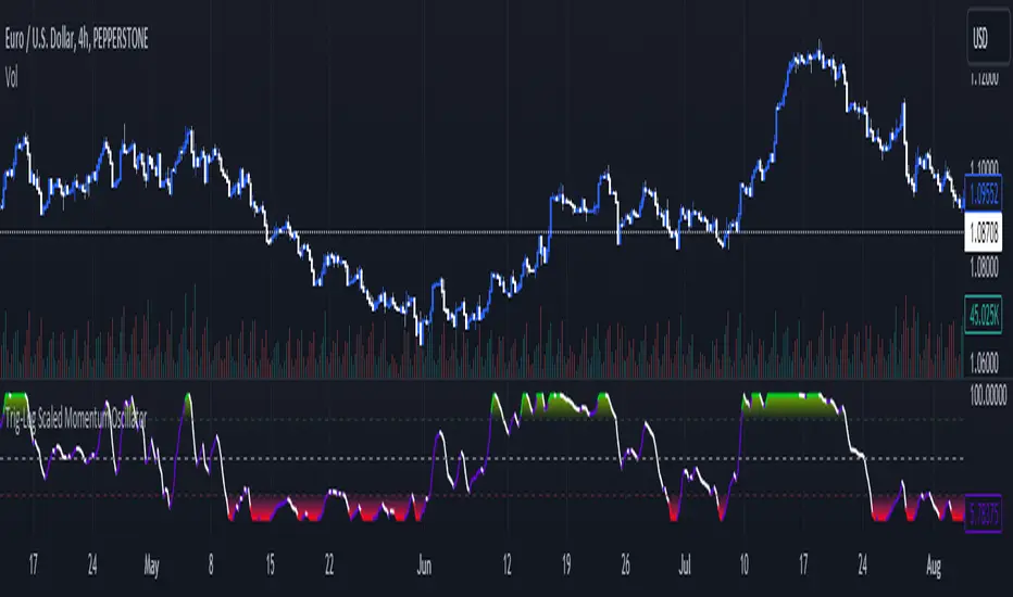
Trig-Log Scaled Momentum Oscillator
Taylor Series Approximations for Trigonometry:
1. The indicator starts by calculating sine and cosine values of the close price using Taylor Series approximations. These approximations use polynomial terms to estimate the values of these trigonometric functions.
Mathematical Component Formation:
2. The calculated sine and cosine values are then multiplied together. This gives us the primary mathematical component, termed as the 'trigComponent'.
Smoothing Process:
3. To ensure that our indicator is less susceptible to market noise and more reactive to genuine price movements, this 'trigComponent' undergoes a smoothing process using a simple moving average (SMA). The length of this SMA is defined by the user.
Logarithmic Transformation:
4. With our smoothed value, we apply a natural logarithm approximation. Again, this approximation is based on the Taylor expansion. This step ensures that all resultant values are positive and offers a different scale to interpret the smoothed component.
Dynamic Scaling:
5. To make our indicator more readable and comparable over different periods, the logarithmically transformed values are scaled between a range. This range is determined by the highest and lowest values of the transformed component over the user-defined 'lookback' period.
ROC (Rate of Change) Direction:
6. The direction of change in our scaled value is determined. This offers a quick insight into whether our mathematical component is increasing or decreasing compared to the previous value.
Visualization:
7. Finally, the indicator plots the dynamically scaled and smoothed mathematical component on the chart. The color of the plotted line depends on its direction (increasing or decreasing) and its boundary values.
오픈 소스 스크립트
트레이딩뷰의 진정한 정신에 따라, 이 스크립트의 작성자는 이를 오픈소스로 공개하여 트레이더들이 기능을 검토하고 검증할 수 있도록 했습니다. 작성자에게 찬사를 보냅니다! 이 코드는 무료로 사용할 수 있지만, 코드를 재게시하는 경우 하우스 룰이 적용된다는 점을 기억하세요.
면책사항
해당 정보와 게시물은 금융, 투자, 트레이딩 또는 기타 유형의 조언이나 권장 사항으로 간주되지 않으며, 트레이딩뷰에서 제공하거나 보증하는 것이 아닙니다. 자세한 내용은 이용 약관을 참조하세요.
오픈 소스 스크립트
트레이딩뷰의 진정한 정신에 따라, 이 스크립트의 작성자는 이를 오픈소스로 공개하여 트레이더들이 기능을 검토하고 검증할 수 있도록 했습니다. 작성자에게 찬사를 보냅니다! 이 코드는 무료로 사용할 수 있지만, 코드를 재게시하는 경우 하우스 룰이 적용된다는 점을 기억하세요.
면책사항
해당 정보와 게시물은 금융, 투자, 트레이딩 또는 기타 유형의 조언이나 권장 사항으로 간주되지 않으며, 트레이딩뷰에서 제공하거나 보증하는 것이 아닙니다. 자세한 내용은 이용 약관을 참조하세요.